3.3 编程实现对数几率回归

参考代码
结合自己的理解，添加注释。

代码

1. 导入相关的库

import numpy as np
import pandas as pd
import matplotlib
from matplotlib import pyplot as plt
from sklearn import linear_model

2. 导入数据，进行数据处理和特征工程

# 1.数据处理，特征工程
data_path = 'watermelon3_0_Ch.csv'
data = pd.read_csv(data_path).values
# 取所有行的第10列(标签列)进行判断
is_good = data[:,9] == '是'
is_bad = data[:,9] == '否'
# 按照数据集3.0α，强制转换数据类型
X = data[:,7:9].astype(float)
y = data[:,9]
y[y=='是'] = 1
y[y=='否'] = 0
y = y.astype(int)

3. 定义若干需要使用的函数
   $$y=\frac{1}{1+e^{-x}}$$

def sigmoid(x):
    """
    构造对数几率函数，它是一种sigmoid函数
    """
    s = 1/(1+np.exp(-x))
    return s

$$\ell (\beta )=\sum _{i=1}^m(-y_i{\beta }^T{\hat{x}}_i+ln(1+e^{{\beta }^T{\hat{x}}_i}))$$

def J_cost(X,y,beta):
    """
    :param X:  sample array, shape(n_samples, n_features)
    :param y: array-like, shape (n_samples,)
    :param beta: the beta in formula 3.27 , shape(n_features + 1, ) or (n_features + 1, 1)
    :return: the result of formula 3.27
    """
    # 构造x_hat，np.c_ 用于连接两个矩阵，规模是（X.row行，X.column+1列）
    X_hat = np.c_[X, np.ones((X.shape[0],1))]
    # β和y均reshape为1列，规模是（X.column+1行，1列）
    beta = beta.reshape(-1,1)
    y = y.reshape(-1,1)
    
    # 计算最大化似然函数的相反数
    L_beta = -y * np.dot(X_hat,beta) + np.log(1+np.exp(np.dot(X_hat,beta)))
    # 返回式3.27的结果
    return  L_beta.sum()

$$\beta =(w;b)$$

def initialize_beta(column):
    """
    初始化β，对应式3.26的假设，规模是（X.column+1行，1列），x_hat规模是（17行，X.column+1列）
    """
    # numpy.random.randn(d0,d1,…,dn)
    # randn函数返回一个或一组样本，具有标准正态分布。标准正态分布又称为u分布，是以0为均值、以1为标准差的正态分布，记为N（0，1）
    # dn表格每个维度
    # 返回值为指定维度的array
    beta = np.random.randn(column+1,1)*0.5+1
    return beta

$$\frac{\partial \ell (\beta )}{\partial \beta }=-\sum _{i=1}^m{\hat{x}}_i(y_i-p_1({\hat{x}}_i;\beta ))$$

def gradient(X,y,beta):
    """
    compute the first derivative of J(i.e. formula 3.27) with respect to beta      i.e. formula 3.30
    计算式3.27的一阶导数
    ----------------------------------------------------
    :param X: sample array, shape(n_samples, n_features)
    :param y: array-like, shape (n_samples,)
    :param beta: the beta in formula 3.27 , shape(n_features + 1, ) or (n_features + 1, 1)
    :return:
    """
    # 构造x_hat，np.c_ 用于连接两个矩阵，规模是（X.row行，X.column+1列）
    X_hat = np.c_[X, np.ones((X.shape[0],1))]
    # β和y均reshape为1列，规模是（X.column+1行，1列）
    beta = beta.reshape(-1,1)
    y = y.reshape(-1,1)
    # 计算p1(X_hat,beta)
    p1 = sigmoid(np.dot(X_hat,beta))
    
    gra = (-X_hat*(y-p1)).sum(0)
    
    return gra.reshape(-1,1) 

$$\frac{{\partial }^2\ell (\beta )}{\partial \beta \partial {\beta }^T}=\sum _{i=1}^m{\hat{x}}_i{\hat{x}}_i^T{p}_1({\hat{x}}_i;\beta )(1-p_1({\hat{x}}_i;\beta ))$$

def hessian(X,y,beta):
    '''
    compute the second derivative of J(i.e. formula 3.27) with respect to beta      i.e. formula 3.31
    计算式3.27的二阶导数
    ----------------------------------
    :param X: sample array, shape(n_samples, n_features)
    :param y: array-like, shape (n_samples,)
    :param beta: the beta in formula 3.27 , shape(n_features + 1, ) or (n_features + 1, 1)
    :return:
    '''
    # 构造x_hat，np.c_ 用于连接两个矩阵，规模是（X.row行，X.column+1列）
    X_hat = np.c_[X, np.ones((X.shape[0],1))]
    # β和y均reshape为1列，规模是（X.column+1行，1列）
    beta = beta.reshape(-1,1)
    y = y.reshape(-1,1)
    # 计算p1(X_hat,beta)
    p1 = sigmoid(np.dot(X_hat,beta))
    
    m,n=X.shape
    # np.eye()返回的是一个二维2的数组(N,M)，对角线的地方为1，其余的地方为0.
    P = np.eye(m)*p1*(1-p1)
    assert P.shape[0] == P.shape[1]
    # X_hat.T是X_hat的转置
    return np.dot(np.dot(X_hat.T,P),X_hat)

使用梯度下降法求解

def update_parameters_gradDesc(X,y,beta,learning_rate,num_iterations,print_cost):
    """
    update parameters with gradient descent method
    """
    for i in range(num_iterations):
        grad = gradient(X,y,beta)
        beta = beta - learning_rate*grad
        
        # print_cost为true时，并且迭代为10的倍数时，打印本次迭代的cost
        if (i%10==0)&print_cost:
            print('{}th iteration, cost is {}'.format(i,J_cost(X,y,beta)))
    
    return beta

def logistic_model(X,y,print_cost=False,method='gradDesc',learning_rate=1.2,num_iterations=1000):
    """
    :param method: str 'gradDesc'or'Newton'
    """
    # 得到X的规模
    row,column = X.shape
    # 初始化β
    beta = initialize_beta(column)
    
    if method == 'gradDesc':
        return update_parameters_gradDesc(X,y,beta,learning_rate,num_iterations,print_cost)
    elif method == 'Newton':
        return update_parameters_newton(X,y,beta,print_cost,num_iterations)
    else:
        raise ValueError('Unknown solver %s' % method)

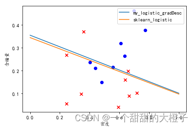
4. 可视化结果

# 1.可视化数据点
# 设置字体为楷体
matplotlib.rcParams['font.sans-serif'] = ['KaiTi']
plt.scatter(data[:, 7][is_good], data[:, 8][is_good], c='b', marker='o') #c参数是颜色，marker是标记
plt.scatter(data[:, 7][is_bad], data[:, 8][is_bad], c='r', marker='x')
# 设置横轴坐标标题
plt.xlabel('密度')
plt.ylabel('含糖量')

# 2.可视化自己写的模型
# 学习得到模型
beta = logistic_model(X,y,print_cost=True,method='gradDesc',learning_rate=0.3, num_iterations=1000)
# 得到模型参数及偏置（截距）
w1, w2, intercept = beta
x1 = np.linspace(0, 1)
y1 = -(w1 * x1 + intercept) / w2
ax1, = plt.plot(x1, y1, label=r'my_logistic_gradDesc')

# 3.可视化sklearn的对率回归模型，进行对比
lr = linear_model.LogisticRegression(solver='lbfgs', C=1000)  # 注意sklearn的逻辑回归中，C越大表示正则化程度越低。
lr.fit(X, y)
lr_beta = np.c_[lr.coef_, lr.intercept_]
print(J_cost(X, y, lr_beta))
# 可视化sklearn LogisticRegression 模型结果
w1_sk, w2_sk = lr.coef_[0, :]
x2 = np.linspace(0, 1)
y2 = -(w1_sk * x2 + lr.intercept_) / w2
ax2, = plt.plot(x2, y2, label=r'sklearn_logistic')
plt.legend(loc='upper right')
plt.show()

可视化结果如下：