MAE源代码理解 part1 : 调试理解法
git官方链接:GitHub - facebookresearch/mae: PyTorch implementation of MAE https//arxiv.org/abs/2111.06377下了MAE代码 完全看不懂 我要一步一步来 把这篇代码给全部理解了 。我自己觉得看大神代码很有用。 这篇文章当笔记用。一,跑示例:怎么说 一上来肯定是把demo里的代码拿出来跑一跑。但是会遇到问题。
目录
git官方链接: GitHub - facebookresearch/mae: PyTorch implementation of MAE https//arxiv.org/abs/2111.06377
下了MAE代码 完全看不懂 我要一步一步来 把这篇代码给全部理解了 。我自己觉得看大神代码很有用。 这篇文章当笔记用。
一,跑示例:
怎么说 一上来肯定是把demo里的代码拿出来跑一跑。但是会遇到问题。 下面时demo的代码。 第一个问题是
TypeError: __init__() got an unexpected keyword argument 'qk_scale'说函数没这个参数 那很简单 找到位置 删掉就行 为啥我敢删 就是因为他的值是 None ,直接删就行
第二个问题是 我一开始把
这三个模型当成了预训练模型 , 下面左就是得到的结果 这啥啊 还原了个寂寞 。 想了半天kaiming是不是错了 ,再想了半天kaiming怎么会错 ,才发现预训练模型藏在链接里。下面这三个只是他开始训练时使用的预训练模型。


链接在demo里找到 两个large的 模型参数如下 跑的结果如上右 对嘛
https://dl.fbaipublicfiles.com/mae/visualize/mae_visualize_vit_large.pth

https://dl.fbaipublicfiles.com/mae/visualize/mae_visualize_vit_large_ganloss.pth
复现结束了 (bushi)
终于把演示跑通了。
2 画图
调试这个方法可太神了,我们上面跑通了demo 就让我们跟着demo一览模型全貌吧!
这段 获取图像并且归一化 然后用plt画出来 这里是先归一化 画图时再返回回来。
(吐槽 : 我不理解 为什么要先归一化 再回来 再画图 多此一举? 我直接show img 不香吗)
# load an image
img_url = 'https://user-images.githubusercontent.com/11435359/147738734-196fd92f-9260-48d5-ba7e-bf103d29364d.jpg' # fox, from ILSVRC2012_val_00046145
# img_url = 'https://user-images.githubusercontent.com/11435359/147743081-0428eecf-89e5-4e07-8da5-a30fd73cc0ba.jpg' # cucumber, from ILSVRC2012_val_00047851
img = Image.open(requests.get(img_url, stream=True).raw)
#raw是一种格式 stream 是确定能下再下。(比如会事先确定内存)
img = img.resize((224, 224))
img = np.array(img) / 255.

assert img.shape == (224, 224, 3)

# normalize by ImageNet mean and std
img = img - imagenet_mean
img = img / imagenet_std

plt.rcParams['figure.figsize'] = [5, 5]   #设置画布尺寸
show_image(torch.tensor(img))

def show_image(image, title=''):
    # image is [H, W, 3]
    assert image.shape[2] == 3
    plt.imshow(torch.clip((image * imagenet_std + imagenet_mean) * 255, 0, 255).int())
    #刚才归一化了 现在返回 记得clip防止越界 int防止小数  因为像素都是整数   imshow竟然可以读张量
    plt.title(title, fontsize=16)
    plt.show()
    plt.axis('off')
    return
3 载入模型
3.1准备模型
chkpt_dir = 'model_save/mae_visualize_vit_large.pth'
model_mae = prepare_model(chkpt_dir, 'mae_vit_large_patch16')
print('Model loaded.')
会进入准备模型的函数里
def prepare_model(chkpt_dir, arch='mae_vit_large_patch16'):
    # build model
    model = getattr(models_mae, arch)()
    # load model
    checkpoint = torch.load(chkpt_dir, map_location='cpu')
    msg = model.load_state_dict(checkpoint['model'], strict=False)
    print(msg)

    return model
对于第一局 getattr(models_mae,arch): 是取models_mae模块里的arch 而这个arch是什么 下图可以看到是一个函数 而且是一个没带括号的函数 (我不理解 ) 所以get后要补一个括号

然后我们进入这个函数, 可以看到这个函数了 哦~ 是一个获取模型的函数 大 中小模型有三个不同的函数 不同函数的参数不一样罢了。

然后就是一个大工程了 我们进这个模型内部看一看。
3.2.1_模型内部
模型代码太大了 我就不贴整个的了 我一部分一部分的贴。
3.2.1.1 编码器模块
from timm.models.vision_transformer import PatchEmbed, Block


self.patch_embed = PatchEmbed(img_size, patch_size, in_chans, embed_dim)
#patch_size 应该是一个图片分出来的 一张有多大  inchans 一般都是3 图片层数嘛
# embed——dim 这个是编出来的特征维度 1024


num_patches = self.patch_embed.num_patches
##num_pathches 大小是x*y 就是图片分成x*y份num_patches = (224/patch_size)**2 = 14 **2 = 196
这个编码 来自于VIT的编码, 然而我并没有看过VIT的代码是什么样子的 。这篇里先不写 ,等到下一篇文章 我就遍历进这个编码函数里 看看是什么东西。 我们就记住 有一个编码的函数 似乎是吧图片 变成一串特征码
self.cls_token = nn.Parameter(torch.zeros(1, 1, embed_dim))
self.pos_embed = nn.Parameter(torch.zeros(1, num_patches + 1, embed_dim),
    requires_grad=False)  # fixed sin-cos embedding
cls令牌 加入 位置编码加入 nn.patameter这个函数 就是将一个不可训练的张量或者矩阵 转换为模型内可以训练的参数。 (想写一个要训练的参数 又不是官方的那些层 ,终于知道方法啦)。cls_token大小是 (1,1,1024) 位置编码是 (1,197,1024) 为啥是197呢 ?应该是为了跟嵌入cls后的编码大小保持一致 然后可以cat 我猜。
        self.blocks = nn.ModuleList([
            Block(embed_dim, num_heads, mlp_ratio, qkv_bias=True, norm_layer=norm_layer)
            for i in range(depth)])
        self.norm = norm_layer(embed_dim)
这里的 block 就是VIT里的那个block 这个block也等到VIT代码时再讲
这里有几个他们用的小trick
nn.LayerNorm   #这个表示在channel 上做归一化
nn.batchNorm  #这个是在batch上归一化
DropPath  # 这个也是一种与dropout不同的 drop方法
nn.GELU   #一种激活函数
nn.ModuleList 其实就是一个列表 把一些块放在这个列表里 与普通列表不同的是 普通的列表不会得到训练 。 这里就是放了24个自注意力块 每个块有12个头 。以上就是编码器用到的模块。
3.2.1.2 解码模块
下面是解码器。
        self.decoder_embed = nn.Linear(embed_dim, decoder_embed_dim, bias=True)
            # 一个fc层 1024到512

        self.mask_token = nn.Parameter(torch.zeros(1, 1, decoder_embed_dim))
            #一个mask编码 (1,1,512)
        self.decoder_pos_embed = nn.Parameter(torch.zeros(1, num_patches + 1,
            decoder_embed_dim), requires_grad=False)  # fixed  sin-cos embedding
              #一个位置编码 而且不训练 (1,197,512)  为什么不训练啊?
        self.decoder_blocks = nn.ModuleList([
            Block(decoder_embed_dim, decoder_num_heads, mlp_ratio, qkv_bias=True, norm_layer=norm_layer)
            for i in range(decoder_depth)])

        self.decoder_norm = norm_layer(decoder_embed_dim)

        self.decoder_pred = nn.Linear(decoder_embed_dim, patch_size**2 * in_chans, bias=True) # decoder to patch
        #预测层  512 到   256*3 (这个也不到224*224*3啊)
解码器的注意力层只有8层 但也是12头的 输入是512维
3.2.1.3 初始化模块
3.2.1.3.1 找位置编码
        self.norm_pix_loss = norm_pix_loss

        self.initialize_weights()
第一个的值是false 等会看看有啥用 第二个是一个函数 我们进去看看 。
       pos_embed = get_2d_sincos_pos_embed(self.pos_embed.shape[-1], int(self.patch_embed.num_patches**.5), cls_token=True)
        self.pos_embed.data.copy_(torch.from_numpy(pos_embed).float().unsqueeze(0))
初始化 第一步 是一个位置编码函数 ,我们进入这个编码函数去看
def get_2d_sincos_pos_embed(embed_dim, grid_size, cls_token=False):
    #embed_dim = 1024 是位置的最后一维 gridSize是每个小patch的长宽 也就是14


    grid_h = np.arange(grid_size, dtype=np.float32)
    grid_w = np.arange(grid_size, dtype=np.float32)
      #生成两个坐标系 14*14的


    grid = np.meshgrid(grid_w, grid_h)  # here w goes first
    #这就是一个坐标系了 不过谁是x 谁是y还要看看
    grid = np.stack(grid, axis=0)
    #  生成了 两个网格。 每个都是14*14  grid现在是(2,14,14)


    grid = grid.reshape([2, 1, grid_size, grid_size])
    #(2,1,14,14)
然后继续进入下层函数 我们继续看 。
    pos_embed = get_2d_sincos_pos_embed_from_grid(embed_dim, grid)


def get_2d_sincos_pos_embed_from_grid(embed_dim, grid):
    assert embed_dim % 2 == 0

    # use half of dimensions to encode grid_h
    emb_h = get_1d_sincos_pos_embed_from_grid(embed_dim // 2, grid[0])  # (H*W, D/2)
    emb_w = get_1d_sincos_pos_embed_from_grid(embed_dim // 2, grid[1])  # (H*W, D/2)

    emb = np.concatenate([emb_h, emb_w], axis=1) # (H*W, D)
    return emb
再进入下层函数 。
def get_1d_sincos_pos_embed_from_grid(embed_dim, pos):


    """
    embed_dim: output dimension for each position   这里只有512
    pos: a list of positions to be encoded: size (M,)    #这里是(1,14,14) 相当于一个通道
    out: (M, D)
    """
    assert embed_dim % 2 == 0
    omega = np.arange(embed_dim // 2, dtype=np.float)
    #    (1,2,3,4.。。。256)
    omega /= embed_dim / 2.
    #这一步是归一化

    omega = 1. / 10000**omega  # (D/2,)
    ##有点像做了个反向 本来是0到1 现在是1到0

    pos = pos.reshape(-1)  # (M,)
    #1,14,14 变成了 196  形式是0到13循环14次
    out = np.einsum('m,d->md', pos, omega)  # (M, D/2), outer product
        #这里是外集 就是一列乘一行 相当于  out就变成 (196, 256)的矩阵了。

    emb_sin = np.sin(out) # (M, D/2)
    emb_cos = np.cos(out) # (M, D/2)

    emb = np.concatenate([emb_sin, emb_cos], axis=1)  # (M, D)

    #对所有值取sin 和cos 之后con起来  但注意维度是1 也就是196*512 前半段是sin 后半段cos
    return emb
下层函数返回后 再次拼起来 变成 196 *1024 这个位置编码真可谓是历尽艰辛 。我们来看 他是怎么来的 。首先 196, 1024分前后两段。看前半段 。 先做个(256,1)长的矩阵 分布再1,256 表示位置 之后呢 再反向后与网格(14*14)拉平后的值做一个外积 这个网格也是位置信息。之后sin 和cos都上 得到两个位置编码。 再拼起来 得到一个维度的编码 。 再把两个维度拼起来得到整体的位置编码。
    if cls_token:
        pos_embed = np.concatenate([np.zeros([1, embed_dim]), pos_embed], axis=0)
    return pos_embed
这里是 将196 1041 , 变成(197,1024) 拼出CLS那一维。
3.2.1.3.2回到初始化
        self.pos_embed.data.copy_(torch.from_numpy(pos_embed).float().unsqueeze(0))
        #将numpy变为tensor 后 转float32 再扩充维度为(1,197,1024) 就得到了编码器的位置编码
  decoder_pos_embed = get_2d_sincos_pos_embed(self.decoder_pos_embed.shape[-1], int(self.patch_embed.num_patches**.5), cls_token=True)
        self.decoder_pos_embed.data.copy_(torch.from_numpy(decoder_pos_embed).float().unsqueeze(0))
解码器的位置编码 (1,197,512) 还是比编码器少了一半
        w = self.patch_embed.proj.weight.data
        torch.nn.init.xavier_uniform_(w.view([w.shape[0], -1]))


        torch.nn.init.normal_(self.cls_token, std=.02)
        torch.nn.init.normal_(self.mask_token, std=.02)
这个w是取出weight层的权重值。 正好可以看出 w的大小是 (1024,3,16,16) 1024是输出维度 3是输入维度 。相当于一个卷积 ? 然后参数进行一个初始化 统一于 (1024, 3*16*16)正太分布
mask 和 cls 也要初始化 。
self.apply(self._init_weights)初始化其他层 self.apply应该是对遍历模型 对每一个模块 使用后面这个函数 我们进入初始化权重函数看一看 ,
    def _init_weights(self, m):
        if isinstance(m, nn.Linear):
            # we use xavier_uniform following official JAX ViT:
            torch.nn.init.xavier_uniform_(m.weight)
            if isinstance(m, nn.Linear) and m.bias is not None:
                nn.init.constant_(m.bias, 0)
        elif isinstance(m, nn.LayerNorm):
            nn.init.constant_(m.bias, 0)
            nn.init.constant_(m.weight, 1.0)
可以看到是如何初始化的 全连接层的 权重使用xavier的均匀分布 偏置设为0
layer归一化层 的偏置为0 权重为1
过程中可以看到对24个注意力层都初始化 而且注意力层里也有各种各样的linear层。

3.2.1.3.3 初始化完成
至此 模型的初始化完成了 我们得到了这个模型。从这些步骤里 我们可以大概看到模型是什么样子的 , 有一个编码器模块 和一个解码器模块。 编码器模块有24层深的16头自注意力模块。 还有一些位置编码和 cls 编码 而解码器只是多了一个mask编码,而且维度会与编码器不一样。
3.3 模型准备完成。
checkpoint = torch.load(chkpt_dir, map_location='cpu')这个chkpt_dir 也就是下载下来的预训练模型 大概应该只是参数 所以需要下面这句 模型载入参数
这里这个strict 意思是 如果与预训练有的层 就使用预训练的参数 模型里 预训练没有的层 就普通初始化。
msg = model.load_state_dict(checkpoint['model'], strict=False)

return model
msg 记录加载的结果 得到完全体模型。
4处理图片
模型准备好了 我们开始用模型处理一个图片看看 。
4.1数据准备
torch.manual_seed(2)   #固定随机数种子
print('MAE with pixel reconstruction:')
run_one_image(img, model_mae)
我们进入了 run_ONE_image函数内部
    x = torch.tensor(img)

    # make it a batch-like
    x = x.unsqueeze(dim=0)
    x = torch.einsum('nhwc->nchw', x)
这里显示了怎么把一个 图片 做成一个batch 第三个einsum 也可以用
torch.transpose() 这个函数来 就是一个维度的转换嘛 把那个3 提到第二维上来。 不过he他们确实精妙 大佬。
loss, y, mask = model(x.float(), mask_ratio=0.75)进入模型运行了 。 从模型返回的是loss 预测值 和mask 我们进模型内部看看 注意模型中运算的值都是float32 格式的 。
latent, mask, ids_restore = self.forward_encoder(imgs, mask_ratio)进froward第一句 就是这一句 我们接下来进入前向编码器里看一看 。
4.2编码步骤
    def forward_encoder(self, x, mask_ratio):
        # embed patches

        x = self.patch_embed(x)  #x:(1,3,224,224)->(1,196,1024)   14*14个片编码

        # add pos embed w/o cls token
        x = x + self.pos_embed[:, 1:, :] # pos是1,197,1024 这里不要0的cls位置  位置信息是直接加到片编码上的  和我的想法很不一样  这样加上来真的会有效果么 。

        # masking: length -> length * mask_ratio
        x, mask, ids_restore = self.random_masking(x, mask_ratio)
    def random_masking(self, x, mask_ratio):
        """
        Perform per-sample random masking by per-sample shuffling.
        Per-sample shuffling is done by argsort random noise.
        x: [N, L, D], sequence
        """
        N, L, D = x.shape  # batch, length, dim
        len_keep = int(L * (1 - mask_ratio))  #计算需要剩余多少片

        noise = torch.rand(N, L, device=x.device)  # noise in [0, 1] noise(1,196)

        # sort noise for each sample
        ids_shuffle = torch.argsort(noise, dim=1)  # ascend: small is keep, large is remove
        # 是对noise的值进行排序  ids_shuffle得到的是下标值。

        ids_restore = torch.argsort(ids_shuffle, dim=1)  #对排序后得到的下标 再排序?这一步#我非常的不懂  后面看
        # keep the first subset
        ids_keep = ids_shuffle[:, :len_keep]    #保持噪声值小的那一堆?
        x_masked = torch.gather(x, dim=1, index=ids_keep.unsqueeze(-1).repeat(1, 1, D))
#这个gather 就是在 x的 dim维 挑index的数。  但是好奇的是 这一串下来 不就是随机挑吗?
# index的维度是 (1,49,1024)X是(1,196,1024) x_masked 是(1,49,1024)

        # generate the binary mask: 0 is keep, 1 is remove
        mask = torch.ones([N, L], device=x.device)
        mask[:, :len_keep] = 0
        #mask 是(1,196) 其中前49都是0 后面都是1

        # unshuffle to get the binary mask
        mask = torch.gather(mask, dim=1, index=ids_restore)
        #到这里终于明白了  这个ids_REStore的作用 就是把mask当成noise 然后把mask按照#restore的位置排序  这样得到的mask就是一个  有mask的地方为1 没mask的地方为0的二维张量。

        return x_masked, mask, ids_restore
这里的mask这里非常难以理解 所以我举个例子 来看看 。
首先 noise是随机生成的 比如说是 noise = [2,0,3,1]
然后 排序argsort: shuffle = [1,3,0,2] 到这里 是为了生成随机数 我们取前两个 也就是随机出来的1,3 作为mask的下标
对shuffle排序 : restore = [2,0,3,1]
mask = [0,0,1,1] 我们根据restore对mask取数 得到[ 1,0,1,0] 下标1,3处就是0. 其实你可以把mask和shuffle看成一样的 你用restore对shuffle 取数 得到【0,1,2,3】发现是排序好的 。 对【1,0,1,0】取数 得到[0,0,1,1]两个是对应起来的。
处理cls
        cls_token = self.cls_token + self.pos_embed[:, :1, :]
        #cls加上位置信息
        cls_tokens = cls_token.expand(x.shape[0], -1, -1)
          # 这一句是为了防止批量的 也就是扩充复制 如果x的batch为N  cls也要复制N份


        x = torch.cat((cls_tokens, x), dim=1)

        #x:(1,50,1024) ->(1,50,1024)   原来是扩充在片数这一维。
这里x要经历24个多头自注意力的磨练 然后归一化。
        for blk in self.blocks:
            x = blk(x)
        x = self.norm(x)
4.3解码步骤
回归forward 来到第二局 解码
pred = self.forward_decoder(latent, ids_restore) # [N, L, p*p*3] def forward_decoder(self, x, ids_restore):
# embed tokens
x = self.decoder_embed(x)
#x (1,50,1024) ->(1,50,512)
# append mask tokens to sequence
mask_tokens = self.mask_token.repeat(x.shape[0], ids_restore.shape[1] + 1 - x.shape[1], 1)
##ids_restore.shape[1] + 1 - x.shape[1] =196+1-50 =147也就是cls加片数减x=需要遮盖数
#self.maskroken.shape = (1,1,512) mask_tokens = (1,147,512) repeate是几就复制几份
x_ = torch.cat([x[:, 1:, :], mask_tokens], dim=1) # no cls token cls辛辛苦苦一辈子
#就这样没了 我还没看到你作用呢 麻烦半天 这里就是完成了 x和mask拼接后的X_
x_ = torch.gather(x_, dim=1, index=ids_restore.unsqueeze(-1).repeat(1, 1, x.shape[2])) # unshuffle 排序回去 按照 mask index.shape = (1,196,512)
x = torch.cat([x[:, :1, :], x_], dim=1) # append cls token 无语
# add pos embed
x = x + self.decoder_pos_embed
# apply Transformer blocks
for blk in self.decoder_blocks:
x = blk(x)
x = self.decoder_norm(x) #就八个 寒酸
# predictor projection
x = self.decoder_pred(x)
#### x (1,197.512) -> (1,197,768)
# remove cls token cls:你有毛病是吧。
x = x[:, 1:, :]
return x得到了模型预测的图像结果
4.4 loss探索
下一步是loss
        pred = self.forward_decoder(latent, ids_restore)  # [N, L, p*p*3]
        loss = self.forward_loss(imgs, pred, mask)
target = self.patchify(imgs)首先进入这个函数 p是一个小图的大小 hw分别是yx方向图的个数 都是14
    def patchify(self, imgs):
        """
        imgs: (N, 3, H, W)
        x: (N, L, patch_size**2 *3)
        """
        p = self.patch_embed.patch_size[0]
        assert imgs.shape[2] == imgs.shape[3] and imgs.shape[2] % p == 0

        h = w = imgs.shape[2] // p
        x = imgs.reshape(shape=(imgs.shape[0], 3, h, p, w, p))
        x = torch.einsum('nchpwq->nhwpqc', x)
        x = x.reshape(shape=(imgs.shape[0], h * w, p**2 * 3))
        return x
x 是(1,3,14,16,14,16) -(1,14,14,16,16,3)
然后reshape (1,14,14,16,16,3) -》(1,196,768) 此中过程 不足为外人道也 鬼知道你咋变的啊 。
target = self.patchify(imgs) 这句就是把原来的图片 也编辑成(1,196,768)大小的
        if self.norm_pix_loss:
            mean = target.mean(dim=-1, keepdim=True)
            var = target.var(dim=-1, keepdim=True)
            target = (target - mean) / (var + 1.e-6)**.5
这个归一化 没进去
可能因为本来已经归过了
        loss = (pred - target) ** 2
        loss = loss.mean(dim=-1)  # [N, L], mean loss per patch
loss是像素差平方 然后对最后一维求平均 变成了 (1,196) 也就是每一个小pat 一个loss
        loss = (loss * mask).sum() / mask.sum()  # mean loss on removed patches
        return loss
mask在相应没有遮盖的地方是0 所以就是只有遮盖的地方才求loss 返回loss值。回到run
4.5 画图
    loss, y, mask = model(x.float(), mask_ratio=0.75)
    y = model.unpatchify(y)
进图unpatchify 根据这个名字 可以看出是吧patch 还原成大图 。
    def unpatchify(self, x):
        """
        x: (N, L, patch_size**2 *3)
        imgs: (N, 3, H, W)
        """
        p = self.patch_embed.patch_size[0]
        h = w = int(x.shape[1]**.5)
        assert h * w == x.shape[1]

        x = x.reshape(shape=(x.shape[0], h, w, p, p, 3))
        x = torch.einsum('nhwpqc->nchpwq', x)
        imgs = x.reshape(shape=(x.shape[0], 3, h * p, h * p))
        return imgs
p 16 h w, 14,14
x (1,196,768) -> (1,14,14,16,16,3) ->(1,3,14,16,14,16) ->imgs(1,3,224,224)
#我忽然想明白了 这里不用知道里面是怎么变化的 只需要操持一致即可 计算机自己就会把他们对应起来 又不用自己管。
回到上面来
    loss, y, mask = model(x.float(), mask_ratio=0.75)
    y = model.unpatchify(y)
    y = torch.einsum('nchw->nhwc', y).detach().cpu()
y(1,3,224,224)- 》(1,224,224,3)
    # visualize the mask
    mask = mask.detach()
    mask = mask.unsqueeze(-1).repeat(1, 1, model.patch_embed.patch_size[0]**2 *3)  # (N, H*W, p*p*3)
    mask = model.unpatchify(mask)  # 1 is removing, 0 is keeping
    mask = torch.einsum('nchw->nhwc', mask).detach().cpu()
mask:(1,196 ) ->(1,196,768) ->(1,3,224,224) ->(1,224,224,3)
x = torch.einsum('nchw->nhwc', x)
# masked image
im_masked = x * (1 - mask)
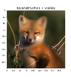
# MAE reconstruction pasted with visible patches
im_paste = x * (1 - mask) + y * maskx (1,3,224,224) ->(1,224,224,3)
1-mask 就是本来是0的 就是没遮盖的变成1 遮盖的变成0 与x相乘 就得到遮盖图片 。
im_paste = x * (1 - mask) + y * mask 遮盖的图片 加上预测的Y与mask相乘 。 因为mask遮盖的地方是1 所以直接相乘
至此得到所有需要画的图像。,
    # make the plt figure larger
    plt.rcParams['figure.figsize'] = [24, 24]

    plt.subplot(1, 4, 1)
    show_image(x[0], "original")

    plt.subplot(1, 4, 2)
    show_image(im_masked[0], "masked")

    plt.subplot(1, 4, 3)
    show_image(y[0], "reconstruction")

    plt.subplot(1, 4, 4)
    show_image(im_paste[0], "reconstruction + visible")

    plt.show()
无语泪凝噎 为啥图不是一块出来的 ????

原来是因为我改了代码

ok 完毕啦 演示结束 改天看其他模块

开放原子开发者工作坊旨在鼓励更多人参与开源活动,与志同道合的开发者们相互交流开发经验、分享开发心得、获取前沿技术趋势。工作坊有多种形式的开发者活动,如meetup、训练营等,主打技术交流,干货满满,真诚地邀请各位开发者共同参与!
更多推荐

 70
70 0
0- 0


 已为社区贡献4条内容

所有评论(0)