基于R语言利用CIBERSORT分析免疫浸润（一）

学习CIBERSORT心得

Kevin丶大牛

7418人浏览 · 2022-07-26 15:57:05

Kevin丶大牛 · 2022-07-26 15:57:05 发布

第一步：认识CIBERSOR

首先我们认识到了单细胞当中每个细胞的特征表达不同。因此对于Bulk数据而言，多个细胞的表达，应该就是这些单个细胞表达的一种加合，我们就可以利用单个细胞的特征使用线性去卷积方法去计算Bulk数据中单细组分含量。

如图，我们可以认为在Sample 1样品中，Cell 1组分含量为a，Cell 2的组分含量为 b。

第二步：CIBERSORT算法

整个算法代码如下，除了此处复制粘贴外，也可以通过网站：https://rdrr.io/github/singha53/amritr/src/R/supportFunc_cibersort.R获取该代码。

补充：也可以使用CIBERSORT的在线工具。

#' CIBERSORT R script v1.03 (last updated 07-10-2015)
#' Note: Signature matrix construction is not currently available; use java version for full functionality.
#' Author: Aaron M. Newman, Stanford University (amnewman@stanford.edu)
#' Requirements:
#'       R v3.0 or later. (dependencies below might not work properly with earlier versions)
#'       install.packages('e1071')
#'       install.pacakges('parallel')
#'       install.packages('preprocessCore')
#'       if preprocessCore is not available in the repositories you have selected, run the following:
#'           source("http://bioconductor.org/biocLite.R")
#'           biocLite("preprocessCore")
#' Windows users using the R GUI may need to Run as Administrator to install or update packages.
#' This script uses 3 parallel processes.  Since Windows does not support forking, this script will run
#' single-threaded in Windows.
#'
#' Usage:
#'       Navigate to directory containing R script
#'
#'   In R:
#'       source('CIBERSORT.R')
#'       results <- CIBERSORT('sig_matrix_file.txt','mixture_file.txt', perm, QN)
#'
#'       Options:
#'       i)  perm = No. permutations; set to >=100 to calculate p-values (default = 0)
#'       ii) QN = Quantile normalization of input mixture (default = TRUE)
#'
#' Input: signature matrix and mixture file, formatted as specified at http://cibersort.stanford.edu/tutorial.php
#' Output: matrix object containing all results and tabular data written to disk 'CIBERSORT-Results.txt'
#' License: http://cibersort.stanford.edu/CIBERSORT_License.txt
#' Core algorithm
#' @param X cell-specific gene expression
#' @param y mixed expression per sample
#' @export
CoreAlg <- function(X, y){

  #try different values of nu
  svn_itor <- 3

  res <- function(i){
    if(i==1){nus <- 0.25}
    if(i==2){nus <- 0.5}
    if(i==3){nus <- 0.75}
    model<-e1071::svm(X,y,type="nu-regression",kernel="linear",nu=nus,scale=F)
    model
  }

  if(Sys.info()['sysname'] == 'Windows') out <- parallel::mclapply(1:svn_itor, res, mc.cores=1) else
    out <- parallel::mclapply(1:svn_itor, res, mc.cores=svn_itor)

  nusvm <- rep(0,svn_itor)
  corrv <- rep(0,svn_itor)

  #do cibersort
  t <- 1
  while(t <= svn_itor) {
    weights = t(out[[t]]$coefs) %*% out[[t]]$SV
    weights[which(weights<0)]<-0
    w<-weights/sum(weights)
    u <- sweep(X,MARGIN=2,w,'*')
    k <- apply(u, 1, sum)
    nusvm[t] <- sqrt((mean((k - y)^2)))
    corrv[t] <- cor(k, y)
    t <- t + 1
  }

  #pick best model
  rmses <- nusvm
  mn <- which.min(rmses)
  model <- out[[mn]]

  #get and normalize coefficients
  q <- t(model$coefs) %*% model$SV
  q[which(q<0)]<-0
  w <- (q/sum(q))

  mix_rmse <- rmses[mn]
  mix_r <- corrv[mn]

  newList <- list("w" = w, "mix_rmse" = mix_rmse, "mix_r" = mix_r)

}

#' do permutations
#' @param perm Number of permutations
#' @param X cell-specific gene expression
#' @param y mixed expression per sample
#' @export
doPerm <- function(perm, X, Y){
  itor <- 1
  Ylist <- as.list(data.matrix(Y))
  dist <- matrix()

  while(itor <= perm){
    #print(itor)

    #random mixture
    yr <- as.numeric(Ylist[sample(length(Ylist),dim(X)[1])])

    #standardize mixture
    yr <- (yr - mean(yr)) / sd(yr)

    #run CIBERSORT core algorithm
    result <- CoreAlg(X, yr)

    mix_r <- result$mix_r

    #store correlation
    if(itor == 1) {dist <- mix_r}
    else {dist <- rbind(dist, mix_r)}

    itor <- itor + 1
  }
  newList <- list("dist" = dist)
}

#' Main functions
#' @param sig_matrix file path to gene expression from isolated cells
#' @param mixture_file heterogenous mixed expression
#' @param perm Number of permutations
#' @param QN Perform quantile normalization or not (TRUE/FALSE)
#' @export
CIBERSORT <- function(sig_matrix, mixture_file, perm=0, QN=TRUE){

  #read in data
  X <- read.table(sig_matrix,header=T,sep="\t",row.names=1,check.names=F)
  Y <- read.table(mixture_file, header=T, sep="\t", row.names=1,check.names=F)

  X <- data.matrix(X)
  Y <- data.matrix(Y)

  #order
  X <- X[order(rownames(X)),]
  Y <- Y[order(rownames(Y)),]

  P <- perm #number of permutations

  #anti-log if max < 50 in mixture file
  if(max(Y) < 50) {Y <- 2^Y}

  #quantile normalization of mixture file
  if(QN == TRUE){
    tmpc <- colnames(Y)
    tmpr <- rownames(Y)
    Y <- preprocessCore::normalize.quantiles(Y)
    colnames(Y) <- tmpc
    rownames(Y) <- tmpr
  }

  #intersect genes
  Xgns <- row.names(X)
  Ygns <- row.names(Y)
  YintX <- Ygns %in% Xgns
  Y <- Y[YintX,]
  XintY <- Xgns %in% row.names(Y)
  X <- X[XintY,]

  #standardize sig matrix
  X <- (X - mean(X)) / sd(as.vector(X))

  #empirical null distribution of correlation coefficients
  if(P > 0) {nulldist <- sort(doPerm(P, X, Y)$dist)}

  #print(nulldist)

  header <- c('Mixture',colnames(X),"P-value","Correlation","RMSE")
  #print(header)

  output <- matrix()
  itor <- 1
  mixtures <- dim(Y)[2]
  pval <- 9999

  #iterate through mixtures
  while(itor <= mixtures){

    y <- Y[,itor]

    #standardize mixture
    y <- (y - mean(y)) / sd(y)

    #run SVR core algorithm
    result <- CoreAlg(X, y)

    #get results
    w <- result$w
    mix_r <- result$mix_r
    mix_rmse <- result$mix_rmse

    #calculate p-value
    if(P > 0) {pval <- 1 - (which.min(abs(nulldist - mix_r)) / length(nulldist))}

    #print output
    out <- c(colnames(Y)[itor],w,pval,mix_r,mix_rmse)
    if(itor == 1) {output <- out}
    else {output <- rbind(output, out)}

    itor <- itor + 1

  }

  #save results
  write.table(rbind(header,output), file="CIBERSORT-Results.txt", sep="\t", row.names=F, col.names=F, quote=F)

  #return matrix object containing all results
  obj <- rbind(header,output)
  obj <- obj[,-1]
  obj <- obj[-1,]
  obj <- matrix(as.numeric(unlist(obj)),nrow=nrow(obj))
  rownames(obj) <- colnames(Y)
  colnames(obj) <- c(colnames(X),"P-value","Correlation","RMSE")
  obj
}

关于算法，我们可以从这些代码中看出CoreAlg，doPerm和CIBERSORT为核心的自定义函数，整个算法是基于线性支持向量回归(SVR)，即进行SVM反卷积推算。

注：SVM和SVR虽然原理类似，但SVM是用作分类，SVR才是用于回归。

理解了整个代码后，我们将其保存为R脚本文件，命名为“Cibersort.R”。方便后续使用。

第三步：准备数据集（LM22.txt和表达谱数据）

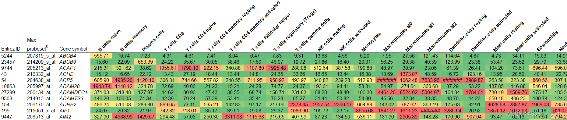
LM22.txt数据集是基准数据库文件，表示22种免疫细胞的marker基因，可以从网站：Robust enumeration of cell subsets from tissue expression profiles | Nature Methods。其中Supplementary information有Supplementary Table 1链接（Leukocyte signature matrix (LM22). Details of LM22, including gene expression matrix and source data. (XLS 424 kb)），成功下载后是.csv文件。我们只需要其中免疫细胞marker基因表达数据，将其提取出来保存为“LM22.txt”文件即可。

至于表达谱数据，进行前期数据清洗，如去除表达量低的基因等，即可用于分析。把处理后的表达谱数据导出为.txt文件，命名为“Data.txt”。

注：CIBERSORT种自带log转换功能，当然也可以对自己的数据集转换。

第四步（最后一步）：CIBERSORT分析

首先加载R脚本文件，然后使用CIBERSORT函数。具体代码如下：

source("Cibersort.R")

result <- CIBERSORT("LM22.txt", "Data.txt", perm = 1000, QN = TRUE)

#perm为置换次数。用于估算单个样本免疫浸润的p值。

#QN为分位数归一化。一般芯片数据设置为T，测序数据设置为F。

注：CIBERSORT算法中自带输出结果代码，默认保存结果文件名为“CIBERSORT-Results.txt”。

到此，关于免疫浸润分析就结束了，关于分析结果的可视化后续进行！