✅博主简介：热爱科研的Matlab仿真开发者，修心和技术同步精进，Matlab项目合作可私信。
🍎个人主页：海神之光
🏆代码获取方式：
海神之光Matlab王者学习之路—代码获取方式
⛳️座右铭：行百里者，半于九十。

更多Matlab仿真内容点击👇
Matlab图像处理（进阶版）
路径规划（Matlab）
神经网络预测与分类（Matlab）
优化求解（Matlab）
语音处理（Matlab）
信号处理（Matlab）
车间调度（Matlab）

⛄一、DCT图像无损压缩简介

1 图像压缩
图像压缩按照压缩过程中是否有信息的损失以及解压后与原始图像是否有误差可以分为无损压缩和有损压缩两大类。无损压缩是指不损失图像质量的压缩，它是对文件的存储方式进行优化，采用某种算法表示重复的数据信息，文件可以完全还原，不会影响文件内容。一般来说，由于无损压缩只是删除了图像数据中的冗余信息，可以准确地恢复原始图像，所以不可能达到很高的压缩比。有损压缩是指损失图像质量的压缩，它将不相干的信息也删除了，因此解压时只能将原始图像进行近似的还原，它的高压缩比是以牺牲图像质量为代价的。

2 JPRG图像压缩
JPEG 提出的 JPEG 标准是为连续色调图像的压缩提供的公共标准。连续色调图像并不局限于单色调( 黑白) 图像，该标准可适用于各种多媒体存储和通信应用所使用的灰度图像、摄影图像及静止视频压缩文件。
JPEG 标准还提出:
①必须将图像质量控制在可视保真度高的范围内，同时编码器可被参数化，允许设置压缩或质量水平
②压缩标准可以应用于任何一类连续色调数字图像，并不应受到维数、颜色、画面尺寸、内容和色调的限制
③压缩标准必须从完全无损到有损范围内可选，以适应不同的存储 CPU 和显示要求

图像压缩编码方法从压缩编码算法原理上可以分为无损压缩编码、有损压缩编码、混合编码方法。而JPEG 标准就是一种混合编码方法，既有无损的压缩编码又有有损的压缩编码。有损压缩方法是以 DCT 变换为基础的压缩方法，其压缩率比较高，是JPEG 标准的基础。无损压缩方法又称预测压缩方法，是以二维 DPCM 为基础的压缩方式，解码后能完全精确地恢复原图像采样值，其压缩比低于有损压缩方法。

观察下图中的编码器负责降低输入图像的编码、像素间和心理视觉冗余。在编码处理的第一阶段，离散余弦变换器将输入图像变换成一种( 通常不可见的) 格式，以便减少像素间的冗余。在第二阶段，量化器根据预定义的保真度准则来减少映射变换器输出的精确性，以便试图去除心理视觉冗余数据。这种操作是不可逆的，当进行无损压缩时，则必须将其忽略。在第三个即最后一个处理阶段，熵编码器根据所用的码字对量化器输出和离散余弦变换输出创建码字( 减少编码冗余）。

3 二维离散余弦变换
离散余弦变换(Discrete Cosine Transform),简称DCT变换.是一种与傅立叶变换紧密相关的数学运算.在傅立叶级数展开式中，如果被展开的函数是实偶函数，那么其傅立叶级数中只包含余弦项,再将其离散化可导出余弦变换，因此称之为离散余弦变换.余弦变换实际上是傅立叶变换的实数部分，其主要用于图像的压缩，目前国际压缩标准的JPEG格式中就用到了DCT变换。
在编码过程中,首先将输入图像颜色空间转换后分解为8× 8大小的数据块，然后用正向二维DCT把每个块转变成64个DCT系数值，其中1个数值是直流(DC)系数，即8× 8空域图像子块的平均值，其余的63个是交流(AC)系数，接下来对DCT系数进行量化，最后将变换得到的量化的DCT系数进行编码和传送，形成压缩后的图像格式。在解码过程中,先对已编码的量化的DCT系数进行解码，然后使用二维DCT反变换求逆量化并把DCT系数转化为8× 8样本像块，最后将操作完成后的块组合成一个单一的图像。这样就完成了图像的压缩和解压过程.研究表明，DCT将8× 8图像块变换为频域时数值集中在左上角，即低频分量都集中在左上角，高频分量分布在右下脚。而低频部分包含了图像大部分信息，相比之下，高频部分包含的信息量较少。为了压缩数据，往往采用忽略高频系数的办法。而较低频系数的修改对原始数据的影响较小。基于DCT的压缩编码属于有损压缩，通过去除图像本身的冗余量和人的视觉冗余量来达到压缩数据的目的，主要分为以下几个步骤:
(1)正向离散余弦变换
(2)量化
(3)Z字形编码
(4)使用差分脉冲编码调制对直流系数进行编码
(5)使用行程长度编码对交流系数进行编码
(6)熵编码
(7)组成位数据流

4 二维DCT变换
二维离散余弦变换的正变换公式为:

在图像的压缩编码中,N一般取8。
二维DCT的反变换公式为:

以上各式中的系数:

5 Matlab调试
根据JPEG 压缩编码算法，要将一幅灰度图像进行压缩编码，首先把图像分成 8* 8 的像素块，分块进行 DCT 变换后，根据 JPEG 标准量化表对变换系数进行量化，再对直流系数( DC) 进行预测编码，对交流系数( AC) 行 zigzag 扫描和可变长编码，然后根据标准的 Huffman 码表进行熵编码，输出压缩图像的比特序列，实现了图像的压缩。
DCT 变换的特点是变换后图像大部分能量集中在左上角，因为左上角反应原图像低频部分数据，右下角反应原图像高频部分数据，而图像的能量通常集中在低频部分。因此 DCT 变换后，只保留 DCT 系数矩阵最左上角的 10 个系数，然后对每个图像块利用这 10个系数进行 DCT 反变换来重构图像。
其基于 DCT 变换矩阵算法的处理过程如下图：

6 Huffman
6.1 什么是Huffman压缩
Huffman( 哈夫曼 ) 算法在上世纪五十年代初提出来了，它是一种无损压缩方法，在压缩过程中不会丢失信息熵，而且可以证明 Huffman 算法在无损压缩算法中是最优的。 Huffman 原理简单，实现起来也不困难，在现在的主流压缩软件得到了广泛的应用。对应用程序、重要资料等绝对不允许信息丢失的压缩场合， Huffman 算法是非常好的选择。

6.2 怎么实现Huffman压缩
哈夫曼压缩是个无损的压缩算法，一般用来压缩文本和程序文件。哈夫曼压缩属于可变代码长度算法一族。意思是个体符号（例如，文本文件中的字符）用一个特定长度的位序列替代。因此，在文件中出现频率高的符号，使用短的位序列，而那些很少出现的符号，则用较长的位序列。

6.3 Huffman编码生成步骤
扫描要压缩的文件，对字符出现的频率进行计算。
把字符按出现的频率进行排序，组成一个队列。
把出现频率最低（权值）的两个字符作为叶子节点，它们的权值之和为根节点组成一棵树。
把上面叶子节点的两个字符从队列中移除，并把它们组成的根节点加入到队列。
把队列重新进行排序。重复步骤 3、4、5 直到队列中只有一个节点为止。
把这棵树上的根节点定义为 0 （可自行定义 0 或 1 ）左边为 0 ，右边为 1 。这样就可以得到每个叶子节点的哈夫曼编码了。

如 (a) 、 (b) 、 © 、 (d) 几个图，就可以将离散型的数据转化为树型的了。
如果假设树的左边用0 表示右边用 1 表示，则每一个数可以用一个 01 串表示出来。

则可以得到对应的编码如下：
1–>110
2–>111
3–>10
4–>0
每一个01 串，既为每一个数字的哈弗曼编码。

6.4 为什么能压缩
压缩的时候当我们遇到了文本中的1 、 2 、 3 、 4 几个字符的时候，我们不用原来的存储，而是转化为用它们的 01 串来存储不久是能减小了空间占用了吗。（什么 01 串不是比原来的字符还多了吗？怎么减少？）大家应该知道的，计算机中我们存储一个 int 型数据的时候一般式占用了 2^32-1 个 01 位，因为计算机中所有的数据都是最后转化为二进制位去存储的。所以，想想我们的编码不就是只含有 0 和 1 嘛，因此我们就直接将编码按照计算机的存储规则用位的方法写入进去就能实现压缩了。
比如：
1这个数字，用整数写进计算机硬盘去存储，占用了 2^32-1 个二进制位
而如果用它的哈弗曼编码去存储，只有110 三个二进制位。
效果显而易见。

6.5 编码实现
编码流程

⛄二、部分源代码

function jpeg

%%%%%%%%%%%%%%%%%%%%%%%%%%%%%%%%%%%%%%%%%%%%%%%%%%%%%%%%%%%%%%%%%%%%%%%%%%%%%%%%%%%%%%%%%%%%%%%%%%%%%%
%%%%%%%%%%%%%%%%%%%%%%%%%%%%%%%%%%%%%%%%%%%%%%%%%%%%%%%%%%%%%%%%%%%%%%%%%%%%%%%%%%%%%%%%%%%%%%%%%%%%%%
%%
%% THIS WORK IS SUBMITTED BY:
%%
%% 紫极神光
%%
%%%%%%%%%%%%%%%%%%%%%%%%%%%%%%%%%%%%%%%%%%%%%%%%%%%%%%%%%%%%%%%%%%%%%%%%%%%%%%%%%%%%%%%%%%%%%%%%%%%%%%
%%%%%%%%%%%%%%%%%%%%%%%%%%%%%%%%%%%%%%%%%%%%%%%%%%%%%%%%%%%%%%%%%%%%%%%%%%%%%%%%%%%%%%%%%%%%%%%%%%%%%%
close all;

% ==================
% section 1.2 + 1.3
% ==================
% the following use of the function:
%
% plot_bases( base_size,resolution,plot_type )
%
% will plot the 64 wanted bases. I will use “zero-padding” for increased resolution
% NOTE THAT THESE ARE THE SAME BASES !
% for reference I plot the following 3 graphs:
% a) 3D plot with basic resolution (64 plots of 8x8 pixels) using “surf” function
% b) 3D plot with x20 resolution (64 plots of 160x160 pixels) using “mesh” function
% c) 2D plot with x10 resolution (64 plots of 80x80 pixels) using “mesh” function
% d) 2D plot with x10 resolution (64 plots of 80x80 pixels) using “imshow” function
%
% NOTE: matrix size of pictures (b),© and (d), can support higher frequency = higher bases
% but I am not asked to draw these (higher bases) in this section !
% the zero padding is used ONLY for resolution increase !
%
% get all base pictures (3D surface figure)
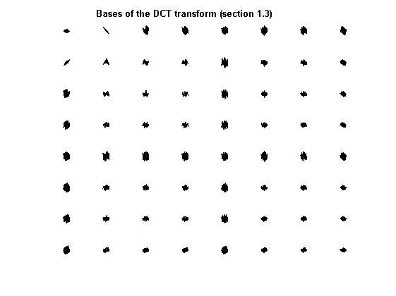
plot_bases( 8,1,‘surf3d’ );

% get all base pictures (3D surface figure), x20 resolution
plot_bases( 8,20,‘mesh3d’ );

% ==================
% section 1.4 + 1.5
% ==================
% for each picture {‘0’…‘9’} perform a 2 dimensional dct on 8x8 blocks.
% save the dct inside a cell of the size: 10 cells of 128x128 matrix
% show for each picture, it’s dct 8x8 block transform.

for idx = 0:9

% load a picture
switch idx
case {0,1}, input_image_128x128 = im2double( imread( sprintf( ‘%d.tif’,idx ),‘tiff’ ) );
otherwise, input_image_128x128 = im2double( imread( sprintf( ‘%d.tif’,idx),‘jpeg’ ) );
end

% perform DCT in 2 dimension over blocks of 8x8 in the given picture
dct_8x8_image_of_128x128{idx+1} = image_8x8_block_dct( input_image_128x128 );

if (mod(idx,2)==0)
figure;
end
subplot(2,2,mod(idx,2)*2+1);
imshow(input_image_128x128);
title( sprintf(‘image #%d’,idx) );
subplot(2,2,mod(idx,2)*2+2);
imshow(dct_8x8_image_of_128x128{idx+1});
title( sprintf(‘8x8 DCT of image #%d’,idx) );
end

% ==================
% section 1.6
% ==================
% do statistics on the cell array of the dct transforms
% create a matrix of 8x8 that will describe the value of each “dct-base”
% over the transform of the 10 given pictures. since some of the values are
% negative, and we are interested in the energy of the coefficients, we will
% add the abs()^2 values into the matrix.
% this is consistent with the definition of the “Parseval relation” in Fourier Coefficients

% initialize the “average” matrix
mean_matrix_8x8 = zeros( 8,8 );

% loop over all the pictures
for idx = 1:10

% transpose the matrix since the order of the matrix is elements along the columns,
% while in the subplot function the order is of elements along the rows
mean_matrix_8x8_transposed = mean_matrix_8x8’;

% make the mean matrix (8x8) into a vector (64x1)
mean_vector = mean_matrix_8x8_transposed(😃;

% sort the vector (from small to big)
[sorted_mean_vector,original_indices] = sort( mean_vector );

% reverse order (from big to small)
sorted_mean_vector = sorted_mean_vector(end👎1);
original_indices = original_indices(end👎1);

% plot the corresponding matrix as asked in section 1.6
figure;
for idx = 1:64
subplot(8,8,original_indices(idx));
axis off;
h = text(0,0,sprintf(‘%4d’,idx));
set(h,‘FontWeight’,‘bold’);
text(0,0,sprintf(’ \n_{%1.1fdb}',20*log10(sorted_mean_vector(idx)) ));
end

% add a title to the figure
subplot(8,8,4);
h = title( ‘Power of DCT coefficients (section 1.6)’ );
set( h,‘FontWeight’,‘bold’ );

% ==================
% section 1.8
% ==================
% picture 8 is chosen
% In this section I will calculate the SNR of a compressed image againts
% the level of compression. the SNR calculation is defined in the header
% of the function: <<calc_snr>> which is given below.
%
% if we decide to take 10 coefficients with the most energy, we will add
% zeros to the other coefficients and remain with a vector 64 elements long
% (or a matrix of 8x8)

% load the original image
original_image = im2double( imread( ‘8.tif’,‘jpeg’ ) );

% I will use this matrix to choose only the wanted number of coefficients
% the matrix is initialized to zeros -> don’t choose any coefficient at all
coef_selection_matrix = zeros(8,8);

% compressed picture set (to show the degrading)
compressed_set = [1 3 5 10 15 20 30 40];

% this loop will choose each time, the “next-most-energetic” coefficient,
% to be added to the compressed image -> and thus to improove the SNR
for number_of_coefficient = 1:64

% find the most energetic coefficient from the mean_matrix
[y,x] = find(mean_matrix_8x8==max(max(mean_matrix_8x8)));

% select if for the compressed image
coef_selection_matrix(y,x) = 1;

% replicate the selection matrix for all the parts of the dct transform
% (remember that the DCT transform creates a set of 8x8 matrices, where
%  in each matrix I need to choose the coefficients defined by the 
%  <<coef_selection_matrix>> matrix )
selection_matrix = repmat( coef_selection_matrix,16,16 );

% set it as zero in the mean_matrix, so that in the next loop, we will
% choose the "next-most-energetic" coefficient
mean_matrix_8x8(y,x) = 0;

% choose the most energetic coefficients from the original image
% (total of <<number_of_coefficient>> coefficients for this run in the loop)
compressed_image = image_8x8_block_dct(original_image) .* selection_matrix;

% restore the compressed image from the given set of coeficients
restored_image = image_8x8_block_inv_dct( compressed_image );

% calculate the snr of this image (based on the original image)
SNR(number_of_coefficient) = calc_snr( original_image,restored_image );

if ~isempty(find(number_of_coefficient==compressed_set))
    if (number_of_coefficient==1)
        figure;
        subplot(3,3,1);
        imshow( original_image );
        title( 'original image' );
    end
    subplot(3,3,find(number_of_coefficient==compressed_set)+1);
    imshow( restored_image );
    title( sprintf('restored image with %d coeffs',number_of_coefficient) );
end

end

%%%%%%%%%%%%%%%%%%%%%%%%%%%%%%%%%%%%%%%%%%%%%%%%%%%%%%%%%%%%%%%%%%%%%%%%%%%%%%%%%%%
%% --------------------------------------------------------------------------------
%% I N N E R F U N C T I O N I M P L E M E N T A T I O N
%% --------------------------------------------------------------------------------
%%%%%%%%%%%%%%%%%%%%%%%%%%%%%%%%%%%%%%%%%%%%%%%%%%%%%%%%%%%%%%%%%%%%%%%%%%%%%%%%%%%

% ---------------------------------------------------------------------------------
% pdip_dct2 - implementation of a 2 Dimensional DCT
%
% assumption: input matrix is a square matrix !
% ---------------------------------------------------------------------------------
function out = pdip_dct2( in )

% get input matrix size
N = size(in,1);

% build the matrix
n = 0:N-1;
for k = 0:N-1
if (k>0)
C(k+1,n+1) = cos(pi*(2*n+1)k/2/N)/sqrt(N)sqrt(2);
else
C(k+1,n+1) = cos(pi(2n+1)*k/2/N)/sqrt(N);
end
end

out = Cin(C’);

% ---------------------------------------------------------------------------------
% pdip_inv_dct2 - implementation of an inverse 2 Dimensional DCT
%
% assumption: input matrix is a square matrix !
% ---------------------------------------------------------------------------------
function out = pdip_inv_dct2( in )

% get input matrix size
N = size(in,1);

% build the matrix
n = 0:N-1;
for k = 0:N-1
if (k>0)
C(k+1,n+1) = cos(pi*(2*n+1)k/2/N)/sqrt(N)sqrt(2);
else
C(k+1,n+1) = cos(pi(2n+1)*k/2/N)/sqrt(N);
end
end

out = (C’)inC;

% ---------------------------------------------------------------------------------
% plot_bases - use the inverse DCT in 2 dimensions to plot the base pictures
%
% Note: we can get resolution be zero pading of the input matrix !!!
% that is by calling: in = zeros(base_size*resolution)
% where: resolution is an integer > 1
% So I will use zero pading for resolution (same as in the fourier theory)
% instead of linear interpolation.
% ---------------------------------------------------------------------------------

% add a title to the figure
subplot(base_size,base_size,round(base_size/2));
h = title( ‘Bases of the DCT transform (section 1.3)’ );
set( h,‘FontWeight’,‘bold’ );

% ---------------------------------------------------------------------------------
% image_8x8_block_dct - perform a block DCT for an image
% ---------------------------------------------------------------------------------
function transform_image = image_8x8_block_dct( input_image )

% ---------------------------------------------------------------------------------
% image_8x8_block_inv_dct - perform a block inverse DCT for an image
% ---------------------------------------------------------------------------------
function restored_image = image_8x8_block_inv_dct( transform_image )

restored_image = zeros( size( transform_image,1 ),size( transform_image,2 ) );
for m = 0:15
for n = 0:15
restored_image( m8+[1:8],n8+[1:8] ) = …
pdip_inv_dct2( transform_image( m8+[1:8],n8+[1:8] ) );
end
end

% ---------------------------------------------------------------------------------
% calc_snr - calculates the snr of a figure being compressed
%
% assumption: SNR calculation is done in the following manner:
% the deviation from the original image is considered
% to be the noise therefore:
%
% noise = original_image - compressed_image
%
% the SNR is defined as:
%
% SNR = energy_of_image/energy_of_noise
%
% which yields:
%
% SNR = energy_of_image/((original_image-compressed_image)^2)
% ---------------------------------------------------------------------------------

⛄三、运行结果

⛄四、matlab版本及参考文献

1 matlab版本
2014a

2 参考文献
[1] 蔡利梅.MATLAB图像处理——理论、算法与实例分析[M].清华大学出版社，2020.

3 备注
简介此部分摘自互联网，仅供参考，若侵权，联系删除
🍅 仿真咨询
1 各类智能优化算法改进及应用
生产调度、经济调度、装配线调度、充电优化、车间调度、发车优化、水库调度、三维装箱、物流选址、货位优化、公交排班优化、充电桩布局优化、车间布局优化、集装箱船配载优化、水泵组合优化、解医疗资源分配优化、设施布局优化、可视域基站和无人机选址优化

2 机器学习和深度学习方面
卷积神经网络（CNN）、LSTM、支持向量机（SVM）、最小二乘支持向量机（LSSVM）、极限学习机（ELM）、核极限学习机（KELM）、BP、RBF、宽度学习、DBN、RF、RBF、DELM、XGBOOST、TCN实现风电预测、光伏预测、电池寿命预测、辐射源识别、交通流预测、负荷预测、股价预测、PM2.5浓度预测、电池健康状态预测、水体光学参数反演、NLOS信号识别、地铁停车精准预测、变压器故障诊断

3 图像处理方面
图像识别、图像分割、图像检测、图像隐藏、图像配准、图像拼接、图像融合、图像增强、图像压缩感知

4 路径规划方面
旅行商问题（TSP）、车辆路径问题（VRP、MVRP、CVRP、VRPTW等）、无人机三维路径规划、无人机协同、无人机编队、机器人路径规划、栅格地图路径规划、多式联运运输问题、车辆协同无人机路径规划、天线线性阵列分布优化、车间布局优化

5 无人机应用方面
无人机路径规划、无人机控制、无人机编队、无人机协同、无人机任务分配

6 无线传感器定位及布局方面
传感器部署优化、通信协议优化、路由优化、目标定位优化、Dv-Hop定位优化、Leach协议优化、WSN覆盖优化、组播优化、RSSI定位优化

7 信号处理方面
信号识别、信号加密、信号去噪、信号增强、雷达信号处理、信号水印嵌入提取、肌电信号、脑电信号、信号配时优化

8 电力系统方面
微电网优化、无功优化、配电网重构、储能配置

9 元胞自动机方面
交通流 人群疏散 病毒扩散 晶体生长

10 雷达方面
卡尔曼滤波跟踪、航迹关联、航迹融合