RGB空间中的彩色图像分割

⭐️ 为尊重原创性！转载请注明出处：©️ Sylvan Ding’s Blog

概述

本文论述了基于欧式距离和曼哈顿距离的彩色图像分割算法，并用python实现了各个算法。之后将二者的优势结合，提出了改进后的曼哈顿距离算法：基于加权曼哈顿距离的彩色图像分割算法，在分割效果和速度上超越了传统的欧式距离分割算法。

核心思想

在一幅RGB图像中分割某个指定的颜色区域（bbox）的物体。给定一个感兴趣的有代表性色彩的彩色样点集，可得到我们希望分割的颜色的“平均”估计。平均彩色用RGB向量$\alpha$表示，分割的目的是将图像中每个RGB像素分类，即在指定的区域内是否有一种颜色。为了执行这一比较，需要有相似性度量：欧氏距离和曼哈顿距离。

欧氏距离

$$D(z,\alpha )=\Vert z-\alpha \Vert ={\left[(z-\alpha {)}^{\mathrm{T}}(z-\alpha )\right]}^{\frac{1}{2}}={\left[{\left(z_R-a_R\right)}^2+{\left(z_G-a_G\right)}^2+{\left(z_B-a_B\right)}^2\right]}^{\frac{1}{2}}$$

其中，下标R、G、B表示向量$\alpha$和$z$的RGB分量。满足$D(z,\alpha )\le D_0$的点的轨道是半径为$D_0$的实心球体，包含在球体内部和表面上的点满足指定的色彩准则。对图像中两组点进行二值化，就产生了一幅二值分割图像。

有时会对欧氏距离进行推广，一种推广形式就是$D(z,\alpha )=[(z-\alpha {)}^T{C}^{-1}(z-\alpha ){]}^{1/2}$，其中$C$是表示我们希望分割的有代表性颜色的样本的协方差矩阵，描述了一个椭球体，其主轴面向最大数据扩展方向。当$C=I_{3\times 3}$时，上式退化为“球形”欧氏距离。

由于欧式距离是正的且单调的，所以可用距离的平方运算来代替，从而避免开方运算，所以我们最终的欧氏距离表达式为：

$$D_E(z,\alpha )=(z-\alpha {)}^T(z-\alpha )$$

曼哈顿距离

但是，上式计算代价较高，故使用曼哈顿距离（RGB空间中的盒边界）可以大幅降低计算代价。其核心思想是在盒中心$\alpha$处，沿每一个颜色轴选择的维数与沿每个轴的样本的标准差成比例，标准差的计算只使用一次样本颜色数据。

单通道曼哈顿距离

在单通道上（以R通道为例），曼哈顿距离的定义为：

$$D_{MR}(z_R,{\alpha }_R)=|z_R-{\alpha }_R|$$

需要满足的色彩准则为：

$$D_{MR}\le \eta {\sigma }_R$$

其中，${\sigma }_R$是样本点红色分量的标准差，$\eta$是标准差的系数，通常取$1.25$。

多通道曼哈顿距离

根据上述定义，多通道平均曼哈顿距离如下：

$$D_M(z,\alpha )=||z-\alpha |{|}_{L1}=|z_R-{\alpha }_R|+|z_G-{\alpha }_G|+|z_B-{\alpha }_B|$$

$$D_M\le \eta ||\sigma |{|}_{L1}$$

其中，$\sigma =({\sigma }_R,{\sigma }_G,{\sigma }_B)$是三通道各自的标准差向量。

多通道曼哈顿距离的改进：带权多通道曼哈顿距离

为R、G、B每个通道设定各自的$\eta$，则需要满足的色彩标准为：

$$D_{MR}\le {\eta }_R{\sigma }_R$$

$$D_{MG}\le {\eta }_G{\sigma }_G$$

$$D_{MB}\le {\eta }_B{\sigma }_B$$

实验和结果分析

import cv2
import numpy as np
import matplotlib.pyplot as plt

img = 'strawberry_color.bmp'
f_bgr = cv2.imread(img, cv2.IMREAD_COLOR)
f_rgb = cv2.cvtColor(f_bgr, cv2.COLOR_BGR2RGB)

bndbox = {'xmin': 3,
          'ymin': 18,
          'xmax': 317,
          'ymax': 344}

f_rec = cv2.rectangle(f_rgb.copy(),
                      (bndbox['xmin'], bndbox['ymin']),
                      (bndbox['xmax'], bndbox['ymax']),
                      color=(255, 255, 0), thickness=5)

plt.imshow(f_rec)
plt.show()

def Euclid(f, box, d0):
    """
    Calculate Euclid distance and return binarized image
    :param f: img
    :param box: (xmin, ymin, xmax, ymax) # VOC format
    :param d0: condition
    :return: binarized image according to condition
    """
    H, W, C = f.shape
    a = np.zeros(C, dtype='float')
    b = np.zeros((H, W), dtype='int')

    for c in range(C):
        a[c] = np.mean(f[box[0]:box[2], box[1]:box[3] ,c])

    a = a.reshape(C, 1)

    for w in range(W):
        for h in range(H):
            z = f[h, w, :].reshape(C, 1)
            d = z - a
            DE = np.dot(d.T, d)
            if DE.sum() <= d0:
                b[h, w] = 1

    return b


def binary_mix(f, b):
    """
    mix input image and binarized image
    :param f: input image
    :param b: its binarized image with only two values 0 and 1
    :return: g
    """
    g = f.copy()
    H, W, C = g.shape

    for c in range(C):
        g[:, :, c] = np.multiply(g[:, :, c], b)

    return g


# Euclid distance

D0_0 = 5000
g_u_b_0 = Euclid(f_rgb, list(bndbox.values()), d0=D0_0)

D0_1 = 10000
g_u_b_1 = Euclid(f_rgb, list(bndbox.values()), d0=D0_1)

fig, axs = plt.subplots(2, 2, figsize=(10, 10))

axs[0][0].set_title('g_u_b_0: D0={}'.format(D0_0))
axs[0][0].imshow(g_u_b_0, cmap='gray')
axs[0][1].set_title('binary_mix(f_rgb, g_u_b_0): D0={}'.format(D0_0))
axs[0][1].imshow(binary_mix(f_rgb, g_u_b_0))

axs[1][0].set_title('g_u_b_1: D0={}'.format(D0_1))
axs[1][0].imshow(g_u_b_1, cmap='gray')
axs[1][1].set_title('binary_mix(f_rgb, g_u_b_1): D0={}'.format(D0_1))
axs[1][1].imshow(binary_mix(f_rgb, g_u_b_1))

plt.suptitle('Euclid distance')
plt.show()

def single_Manhattan(f, box, eta, channel=0):
    """
    Calculate single channel Manhattan distance and return binarized image
    :param f: img
    :param box: (xmin, ymin, xmax, ymax) # VOC format
    :param eta: condition
    :param channel: int, channel number
    :return: binarized image according to condition
    """
    H, W, C = f.shape
    b = np.zeros((H, W), dtype='int')
    c = f[box[0]:box[2], box[1]:box[3] , channel]
    a = np.mean(c)
    sigma = np.std(c)

    for w in range(W):
        for h in range(H):
            z = f[h, w, channel]
            if np.abs(z - a) <= eta * sigma:
                b[h, w] = 1

    return b


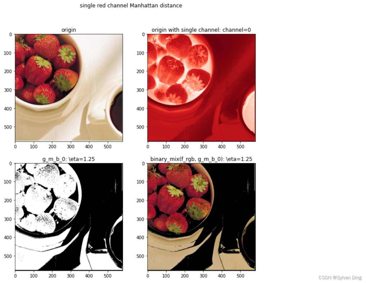
# single red channel Manhattan distance

eta0 = 1.25
channel0 = 0

g_m_b_0 = single_Manhattan(f_rgb, list(bndbox.values()), eta=eta0, channel=channel0)

fig, axs = plt.subplots(2, 2, figsize=(10, 10))

axs[0][0].set_title('origin')
axs[0][0].imshow(f_rgb)
axs[0][1].set_title('origin with single channel: channel={}'.format(channel0))
axs[0][1].imshow(f_rgb[:, :, channel0], cmap='Reds')

axs[1][0].set_title(r'g_m_b_0: \eta={}'.format(eta0))
axs[1][0].imshow(g_m_b_0, cmap='gray')
axs[1][1].set_title(r'binary_mix(f_rgb, g_m_b_0): \eta={}'.format(eta0))
axs[1][1].imshow(binary_mix(f_rgb, g_m_b_0))

plt.suptitle('single red channel Manhattan distance')
plt.show()

基于红色单通道的曼哈顿距离法不能很好地划分背景和草莓，这是因为在红色通道下，背景和草莓的红色值相近（图b说明了这一事实）。

# multi-channel average Manhattan distance

def multi_avg_Manhattan(f, box, eta):
    """
    Calculate multi-channel average Manhattan distance and return binarized image
    :param f: img
    :param box: (xmin, ymin, xmax, ymax) # VOC format
    :param eta: condition
    :return: binarized image according to condition
    """
    H, W, C = f.shape
    a = np.zeros(C, dtype='float')
    sigma = np.zeros(C, dtype='float')
    b = np.zeros((H, W), dtype='int')

    for c in range(C):
        sam = f[box[0]:box[2], box[1]:box[3] ,c]
        a[c] = np.mean(sam)
        sigma[c] = np.std(sam)

    sigmaL1 = np.sum(sigma)

    a = a.reshape(C, 1)

    for w in range(W):
        for h in range(H):
            z = f[h, w, :].reshape(C, 1)
            d = z - a
            DM = np.sum(np.abs(d))
            if DM <= eta * sigmaL1:
                b[h, w] = 1

    return b


eta1 = 1.1

g_m_b_1 = multi_avg_Manhattan(f_rgb, list(bndbox.values()), eta=eta1)

fig, axs = plt.subplots(1, 2, figsize=(10, 5))

axs[0].set_title(r'g_m_b_1: \eta={}'.format(eta1))
axs[0].imshow(g_m_b_1, cmap='gray')
axs[1].set_title(r'binary_mix(f_rgb, g_m_b_1): \eta={}'.format(eta1))
axs[1].imshow(binary_mix(f_rgb, g_m_b_1))

plt.suptitle('multi-channel average Manhattan distance')
plt.show()

可以看到，"平均多通道"曼哈顿法优于"红色单通道"曼哈顿法。

def multi_weight_Manhattan(f, box, etas):
    """
    Calculate multi-channel weighted Manhattan distance and return binarized image
    :param f: img
    :param box: (xmin, ymin, xmax, ymax) # VOC format
    :param etas: conditions for each channel like (eta0, eta1, eta2)
    :return: binarized image according to condition
    """
    H, W, C = f.shape
    bs = np.zeros_like(f, dtype='int') # bs is the valid binarized matrix for each channel of f

    for c in range(C):
        bs[:, :, c] = single_Manhattan(f, box, etas[c], c)

    b = np.sum(bs, axis=2)

    for w in range(W):
        for h in range(H):
            if b[w, h] == C:
                temp = 1
            else:
                temp = 0
            b[w, h] = temp

    return b


# RGB

fig, axs = plt.subplots(1, 3, figsize=(10, 4))

axs[0].set_title('R')
axs[0].imshow(f_rgb[:, :, 0], cmap='gray')
axs[1].set_title('G')
axs[1].imshow(f_rgb[:, :, 1], cmap='gray')
axs[2].set_title('B')
axs[2].imshow(f_rgb[:, :, 2], cmap='gray')

plt.suptitle('RGB')
plt.show()

# multi-channel weighted Manhattan distance

eta2 = (1.4, 1.1, 1.3)

g_m_b_2 = multi_weight_Manhattan(f_rgb, list(bndbox.values()), etas=eta2)

fig, axs = plt.subplots(1, 2, figsize=(10, 5))

axs[0].set_title('g_m_b_2')
axs[0].imshow(g_m_b_2, cmap='gray')
axs[1].set_title('binary_mix(f_rgb, g_m_b_2)')
axs[1].imshow(binary_mix(f_rgb, g_m_b_2))

plt.suptitle(r'multi-channel weighted Manhattan distance: \etas={}'.format(str(eta2)))
plt.show()

使用多通道加权曼哈顿距离法，极大提升了计算的效率，并且获得了近似、甚至优于欧几里得距离法的结果！

参考文献

1. 数字图像处理：第3版，北京：电子工业出版社