【Pytorch】整体工作流程代码详解(新手入门)
本文介绍Pytorch的基本工作流程及代码,以及如何在GPU上训练模型,包括数据准备、模型搭建、模型训练、评估及模型的保存和载入。适合有一定的Python和机器学习基础的深度学习/Pytorch初学者。
一、前言
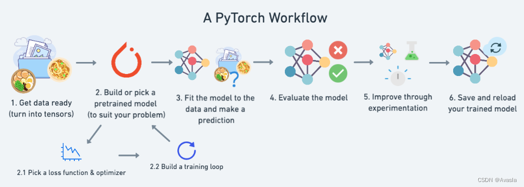
本文详细介绍Pytorch的基本工作流程及代码,以及如何在GPU上训练模型(如下图所示)包括数据准备、模型搭建、模型训练、评估及模型的保存和载入。
适用读者:有一定的Python和机器学习基础的深度学习/Pytorch初学者。

本文内容:
- 一、前言
- 二、环境配置说明
- 三、步骤详细说明
- 1. 数据准备 (Data Pre)
- 1.1 导入包
- 1.2 生成数据集 & 数据集切分
- 1.3 数据可视化
- 2. 模型搭建(Building Model)
- 2.1 创建模型
- 2.2 训练前的模型表现
- 3. 模型训练(Training Model)
- 3.1 损失函数和优化器(Loss function & optimizer)
- 3.2 训练&测试循环(Training/Testing Loop)
- 4. 模型评估
- 5. 保存和导入模型
- 5.1 保存/导出模型
- 5.2 读取/导入模型
- 5.2.1 模型导入
- 5.2.2 检验导入模型
- 四、步骤汇总(在GPU上运算)
- 1. 数据准备
- 2. 建立Pytorch线性模型
- 3. 模型训练
- 4. 模型评估
- 5. 保存&载入模型
- 五、核心代码总结
- 1. 模型搭建
- 2. 模型训练
- 3. 模型评估
- 4. 模型保存和载入
- 5.GPU设置相关
- 参考资料
二、环境配置说明
整体代码在Colab上运行 (需要科学上网),设置为GPU。
GPU 设置步骤如下:


三、步骤详细说明
1. 数据准备 (Data Pre)
1.1 导入包
import torch
from torch import nn # 该模块提供了许多用于定义神经网络层函数和类。
import matplotlib.pyplot as plt

# 检查版本
torch.__version__
1.2 生成数据集 & 数据集切分
# 设置初始参数
weight = 0.7
bias = 0.3

# 创建数据
start = 0
end = 1
step = 0.02
X = torch.arange(start, end, step).unsqueeze(dim=1)
y = weight * X + bias

# 数据集切分
train_split = int(0.8 * len(X))
X_train, y_train = X[:train_split], y[:train_split]
X_test, y_test = X[train_split:], y[train_split:]

len(X_train), len(y_train), len(X_test), len(y_test)
1.3 数据可视化
# 自定义一个画图功能
def plot_predictions(train_data=X_train,
           train_labels=y_train,
           test_data=X_test,
           test_labels=y_test,
           predictions=None):

  plt.figure(figsize=(10, 7))
  plt.scatter(train_data, train_labels, c="b", s=4, label="Training data") # 蓝色为训练集
  plt.scatter(test_data, test_labels, c="g", s=4, label="Testing data") # 绿色是测试集

  if predictions is not None:
    #红色标预测数据
    plt.scatter(test_data, predictions, c="r", s=4, label="Predictions")
  plt.legend(prop={"size": 14});

#查看数据图
plot_predictions();

2. 模型搭建(Building Model)
| PyTorch模块 | 作用 |
|---|---|
torch.nn | 包含了计算图的所有构建模块(本质上是按特定方式执行的一系列计算)。 |
torch.nn.Parameter | 存储可以与nn.Module一起使用的张量。如果requires_grad=True,则会自动计算梯度(用于通过梯度下降更新模型参数),通常称为“autograd”。 |
torch.nn.Module | 所有神经网络模块的基类,所有神经网络的构建模块都是它的子类。如果你在 PyTorch 中构建神经网络,你的模型应该是nn.Module的子类。需要实现一个forward()方法。 |
torch.optim | 包含各种优化算法(告诉存储在nn.Parameter中的模型参数如何改变以改进梯度下降,从而减少损失)。 |
def forward() | 所有nn.Module子类都需要一个forward()方法,它定义了在传递给特定nn.Module的数据上将进行的计算(例如上面的线性回归公式)。 |
如果上述内容听起来复杂,可以这样理解,几乎所有 PyTorch 神经网络中的组件都来自torch.nn:
nn.Module包含更大的构建模块(层)nn.Parameter包含较小的参数,如权重和偏差(将它们组合在一起以创建nn.Module)forward()告诉较大的模块如何对输入(充满数据的张量)进行计算torch.optim包含优化方法,用于改进nn.Parameter中的参数以更好地表示输入数据
2.1 创建模型
# 创建一个线性回归模型类
class LinearRegressionModel(nn.Module):
    def __init__(self):
        super().__init__()
        #权重参数
        self.weights = nn.Parameter(torch.randn(1, # 从随机权重开始(这将随着模型学习而调整)
                      dtype=torch.float), # PyTorch 默认使用 float32
                      requires_grad=True) # <- can we update this value with gradient descent?)
        #偏差参数
        self.bias = nn.Parameter(torch.randn(1,
                    dtype=torch.float),
                    requires_grad=True)

    # forward 方法定义了模型中的计算过程
    def forward(self, x: torch.Tensor) -> torch.Tensor: # "x" 是输入数据(例如训练/测试特征)
        return self.weights * x + self.bias # 这是线性回归公式(y = m*x + b)
requires_grad=True在这里怎么理解?
requires_grad是一个用于跟踪张量是否需要计算梯度的标志。如果这个张量需要计算梯度,则为 True,否则为 False。
在例子中,设置
requires_grad=True
会告诉PyTorch跟踪权重和偏差的梯度,并在进行反向传播和优化时使用这些梯度来更新它们的值,以便最小化模型的训练误差。参考链接:https://pytorch.org/docs/stable/generated/torch.Tensor.requires_grad.html
2.2 训练前的模型表现
随机初始化模型参数的值,并且查看训练前,该模型的表现情况
# 设置种子,因为 nn.Parameter 是随机初始化的
torch.manual_seed(42) # 如果注释掉这行,每次重复运行的结果会不一样

# 创建一个模型model_0
model_0 = LinearRegressionModel()

# 检查nn.Module 中的 nn.Parameter
list(model_0.parameters())

# 列出模型中的参数
model_0.state_dict()

# 模型预测
with torch.inference_mode():
    y_preds = model_0(X_test)

# Note: 在老版本中可能会使用 torch.no_grad()
# with torch.no_grad():
#   y_preds = model_0(X_test)

# 查看预测结果
print(f"Number of testing samples: {len(X_test)}")
print(f"Number of predictions made: {len(y_preds)}")
print(f"Predicted values:\n{y_preds}")

plot_predictions(predictions=y_preds)

#查看预测结果偏差情况
y_test - y_preds

3. 模型训练(Training Model)
3.1 损失函数和优化器(Loss function & optimizer)
# 损失函数
loss_fn = nn.L1Loss() # MAE = L1Loss

# 优化器
optimizer = torch.optim.SGD(params=model_0.parameters(), lr=0.01)
优化器是什么?
- 在机器学习中,优化器(optimizer)是用于最小化或最大化目标函数的算法。它们被用于调整模型中可调参数的值,以便使模型能够更好地拟合训练数据。
- 优化器根据计算出的损失函数的梯度来更新模型参数。梯度指向损失函数增长最快的方向,因此优化器通过沿着梯度的相反方向更新模型参数,以便在训练过程中逐步减少损失函数的值。
- 常见的优化器包括随机梯度下降(SGD)、动量优化器(Momentum)、AdaGrad、RMSprop、以及Adam 等。 每种优化器都有自己的更新规则和超参数,因此在选择优化器时需要考虑模型的特性以及训练数据的特点。
在上面代码中,参数如下所示:
torch.optim.SGD:这是一个使用随机梯度下降(Stochastic Gradient Descent,SGD)算法进行优化的优化器。model.parameters():这是要优化的模型参数的列表。通过将模型的参数传递给优化器,优化器可以使用梯度下降算法来更新这些参数。lr=0.01:这是学习率(learning rate)的值,它决定了每次更新模型参数时的步长大小。学习率越大,模型参数更新得越快,但可能会错过最优解;学习率越小,模型参数更新得越慢,但可能更接近最优解。
3.2 训练&测试循环(Training/Testing Loop)
对于训练循环,可以一共分成下面5个步骤:
| 步骤名称 | 功能 | 代码示例 |
|---|---|---|
| 1. 前向传播 | 模型对所有训练数据进行一次计算,执行其forward()函数计算。 | model(x_train) |
| 2 .计算损失 | 将模型的输出(预测值)与实际值进行比较,并评估它们的误差程度。 | loss = loss_fn(y_pred, y_train) |
| 3 . 清除梯度 | 将优化器的梯度设置为零(它们默认会累积),以便可以针对特定训练步骤重新计算。 | optimizer.zero_grad() |
| 4 . 对损失进行反向传播 | 计算损失相对于每个需要更新的模型参数的梯度(每个参数都要设置requires_grad=True)。这就是所谓的反向传播,因此称为“向后”。 | loss.backward() |
| 5 . 更新优化器(梯度下降) | 根据损失梯度更新requires_grad=True的参数,以改进它们。 | optimizer.step() |
注意!测试循环不包括执行反向传播(loss.backward())或更新优化器(optimizer.step()),这是因为在测试过程中模型的参数不会发生变化,它们已经被计算过了。在测试过程中,我们只对模型通过前向传递产生的输出感兴趣。
torch.manual_seed(42)

epochs=100

train_loss_values=[]
test_loss_values=[]
epoch_count=[]

for epoch in range(epochs):
  model_0.train() # 将模型置于训练模式

  #1.前向传播,在训练数据上进行前向传递,使用模型内部的 forward() 方法。
  y_pred=model_0(X_train)

  #2.计算损失
  loss=loss_fn(y_pred,y_train)

  #3.清除梯度,将有害器的梯度设置为0
  optimizer.zero_grad()

  #4.对损失进行反向传播
  loss.backward()

  #5.更新优化器
  optimizer.step()

  ## 测试

  model_0.eval # 将模型置于评估模式

  with torch.inference_mode():
    #1.在测试数据上进行钱箱传播
    test_pred=model_0(X_test)

    #2.计算损失
    # 预测结果采用 `torch.float` 数据类型,因此需要使用相同类型的张量。
    test_loss=loss_fn(test_pred,y_test.type(torch.float))

    #结果输出
    if epoch % 10==0:
      epoch_count.append(epoch)
      train_loss_values.append(loss.detach().numpy())
      test_loss_values.append(test_loss.detach().numpy())
      print(f"Epoch: {epoch} | MAE Train Loss: {loss} |MAE Test Loss:{test_loss}")
下面结果可以看出,通过10次训练之后,误差大大降低了。
#损失结果可视化
plt.plot(epoch_count, train_loss_values, label="Train loss")
plt.plot(epoch_count, test_loss_values, label="Test loss")
plt.title("Training and test loss curves")
plt.ylabel("Loss")
plt.xlabel("Epochs")
plt.legend();

# 输出学习后的参数
print("The model learned the following values for weights and bias:")
print(model_0.state_dict())
print("\nAnd the original values for weights and bias are:")
print(f"weights: {weight}, bias: {bias}")

虽然损失降低了,但是最终输出的参数和真实的还是有一定差异。
4. 模型评估
在使用PyTorch模型进行预测(也称为执行推断)时,有三件事需要记住:
- 将模型设置为评估模式(
model.eval())。 - 使用
with torch.inference_mode():…。 - 所有预测都应该使用相同设备上的对象(例如,仅在GPU上使用数据和模型,或仅在CPU上使用数据和模型)。
前两项确保在训练过程中PyTorch在幕后使用的所有有用的计算和设置都被关闭(这会加快计算速度)。第三项确保不会遇到跨设备错误。
# 1. 将模型设置为评估模式
model_0.eval()

# 2. 设置torch.inference_mode():
with torch.inference_mode():
  # 3. 确保模型和数据在同一设备上进行计算
  # 在这个例子中,我们的数据和模型默认都在 CPU 上。
  # model_0.to(device)
  # X_test = X_test.to(device)
  y_preds = model_0(X_test)

y_preds

plot_predictions(predictions=y_preds)

和之前的图对比,预测结果大大提升。
5. 保存和导入模型
在实际训练过程中,我们可能会在Google Colab或带有GPU的本地计算机上训练模型,但最终希望将其导出到某种应用程序中供他人使用;或者,希望暂时保存模型的进度,并稍后加载它。
对于在PyTorch中保存和加载模型,有三种主要方法:
| PyTorch方法 | 功能 |
|---|---|
| torch.save | 使用pickle将序列化对象保存到磁盘。可以使用torch.save保存模型、张量和各种其他Python对象,例如字典。 |
| torch.load | 使用pickle的反序列化功能可以反序列化和加载已完成序列化的Python对象文件(如模型、张量或字典)到内存中。还可以设置要将对象加载到的设备(CPU、GPU等)。 |
| torch.nn.Module.load_state_dict | 使用保存的state_dict()对象加载模型的参数字典(model.state_dict())。 |
5.1 保存/导出模型
torch.save(obj, f)语法介绍:
- obj 是目标模型的参数
state_dict() - f 是保存路径
from pathlib import Path

# 1. 创建模型字典
MODEL_PATH = Path("models")
MODEL_PATH.mkdir(parents=True, exist_ok=True)

# 2. 创建模型保存路径
MODEL_NAME = "01_pytorch_workflow_model_0.pth" #保存格式以.pt或.pth后缀结尾
MODEL_SAVE_PATH = MODEL_PATH / MODEL_NAME

# 3. 保存模型参数
print(f"Saving model to: {MODEL_SAVE_PATH}")
torch.save(obj=model_0.state_dict(), # 只保存state_dict();只保存训练后的模型参数
           f=MODEL_SAVE_PATH)
5.2 读取/导入模型
5.2.1 模型导入
下面的代码中
直接在torch.nn.Module.load_state_dict()内部调用torch.load()
因为我们只保存了模型的state_dict(),它是一个包含学习参数的字典,而不是整个模型,
所以我们首先必须使用torch.load()加载参数state_dict(),然后将该state_dict()传递给模型。
为什么不保存整个模型呢?
虽然保存整个模型(包含参数)看起来更加直接简单,但这种方法在重构后会引起各种方式的中断。
- 官方解释如下:
The disadvantage of this approach is that the serialized data is bound to the specific classes and the exact directory structure used when the model is saved. The reason for this is because pickle does not save the model class itself. Rather, it saves a path to the file containing the class, which is used during load time. Because of this, your code can break in various ways when used in other projects or after refactors.因此,我们使用灵活的方法仅保存和加载
state_dict(),它基本上是一个模型参数的字典。
下面我们通过创建LinearRegressionModel的另一个实例来测试一下,它是torch.nn.Module的子类,因此具有内置的load_state_dict()方法。
# 加载模型
loaded_model_0 = LinearRegressionModel()

# 加载保存的state_dict(这将用训练好的权重参数更新模型)
loaded_model_0.load_state_dict(torch.load(f=MODEL_SAVE_PATH))
5.2.2 检验导入模型
# 1. 模型调为测试模式
loaded_model_0.eval()

# 2. 预测结果
with torch.inference_mode():
    loaded_model_preds = loaded_model_0(X_test)

# 3. 对比结果:判断原预测结果是否和导入模型的预测结果一致
y_preds == loaded_model_preds

四、步骤汇总(在GPU上运算)
import torch
from torch import nn
import matplotlib.pyplot as plt

# torch.__version__```

# 设置设备为GPU(如果可用),否则为CPU。
device = "cuda" if torch.cuda.is_available() else "cpu"
print(f"Using device: {device}")
1. 数据准备
weight = 0.7
bias = 0.3

start = 0
end = 1
step = 0.02

X = torch.arange(start, end, step).unsqueeze(dim=1)
y = weight * X + bias
X[:10], y[:10]

# Split data
train_split = int(0.8 * len(X))
X_train, y_train = X[:train_split], y[:train_split]
X_test, y_test = X[train_split:], y[train_split:]

len(X_train), len(y_train), len(X_test), len(y_test)
2. 建立Pytorch线性模型
这里我们直接使用 nn.Linear(in_features, out_features) 构建模型。
其中,in_features 是输入数据的维度数量,而 out_features 是输出的维度数量。
在我们的例子中,这两者都是 1,因为我们的数据每个标签(y)有 1 个输入特征(X)。

class LinearRegressionModelV2(nn.Module):
    def __init__(self):
        super().__init__()
        # 使用nn.Linear()
        self.linear_layer = nn.Linear(in_features=1,
                        out_features=1)
    # 定义forward
    def forward(self, x: torch.Tensor) -> torch.Tensor:
        return self.linear_layer(x)

torch.manual_seed(42)
model_1 = LinearRegressionModelV2()
model_1, model_1.state_dict()

# 检查现在的设备
next(model_1.parameters()).device
当前使用的是CPU
# 设置设备为GPU(如果可用),否则为CPU。
device
model_1.to(device) # 设置设备
next(model_1.parameters()).device #再检查设备
已经转移到GPU上了
3. 模型训练
# 损失函数和优化器
loss_fn = nn.L1Loss()
optimizer = torch.optim.SGD(params=model_1.parameters(),
                            lr=0.01)
要注意把训练和测试数据都转移到GPU上面,因为上一步,我们已经把模型设置在GPU上了。
torch.manual_seed(42)
epochs = 1000

# 将数据放置在可用的设备上。
# 如果没有这样做,会出现错误(并非所有模型/数据都在设备上
X_train = X_train.to(device)
X_test = X_test.to(device)
y_train = y_train.to(device)
y_test = y_test.to(device)

for epoch in range(epochs):
    model_1.train()
    y_pred = model_1(X_train)
    loss = loss_fn(y_pred, y_train)
    optimizer.zero_grad()
    loss.backward()
    optimizer.step()

    ### Testing
    model_1.eval()
    with torch.inference_mode():
        test_pred = model_1(X_test)
        test_loss = loss_fn(test_pred, y_test)

    if epoch % 100 == 0:
        print(f"Epoch: {epoch} | Train loss: {loss} | Test loss: {test_loss}")

from pprint import pprint # pprint = pretty print, see: https://docs.python.org/3/library/pprint.html
print("The model learned the following values for weights and bias:")
pprint(model_1.state_dict())
print("\nAnd the original values for weights and bias are:")
print(f"weights: {weight}, bias: {bias}")

从参数结果可见,模型的参数(0.6968,0.3025)已经基本和实际参数(0.7,0.3)一致了。
4. 模型评估
在查看结果时,也要注意数据的位置,比如plot_predictions(predictions=y_preds)会因为数据不在CPU上而失效。
model_1.eval()
with torch.inference_mode():
    y_preds = model_1(X_test)
y_preds

# plot_predictions(predictions=y_preds) # 原来的代码失效了,因为现在数据不在CPU上

# 将数据放到CPU上并且作图
plot_predictions(predictions=y_preds.cpu())

现在模型的预测结果和实际一致。
5. 保存&载入模型
导出和导入的方法基本没变,但是要注意导入时,模型所在的位置。
5.1 模型导出
# 导出
from pathlib import Path

MODEL_PATH = Path("models")
MODEL_PATH.mkdir(parents=True, exist_ok=True)

MODEL_NAME = "01_pytorch_workflow_model_1.pth"
MODEL_SAVE_PATH = MODEL_PATH / MODEL_NAME

print(f"Saving model to: {MODEL_SAVE_PATH}")
torch.save(obj=model_1.state_dict(),f=MODEL_SAVE_PATH)
5.2 模型导入
#导入
loaded_model_1 = LinearRegressionModelV2()

loaded_model_1.load_state_dict(torch.load(MODEL_SAVE_PATH))

# 将模型放到目标设备上
loaded_model_1.to(device)

print(f"Loaded model:\n{loaded_model_1}")
print(f"Model on device:\n{next(loaded_model_1.parameters()).device}")

模型在CPU上。
5.3 导入模型检查
# 导入模型预测结果检查
loaded_model_1.eval()
with torch.inference_mode():
    loaded_model_1_preds = loaded_model_1(X_test)

#检查载入模型是否和原模型结果一致
y_preds == loaded_model_1_preds
预测结果一致

五、核心代码总结
1. 模型搭建
nn.Module包含更大的构建模块(层)nn.Parameter包含较小的参数,如权重和偏差(将它们组合在一起以创建nn.Module)forward()告诉较大的模块如何对输入(充满数据的张量)进行计算torch.optim包含优化方法,用于改进nn.Parameter中的参数以更好地表示输入数据
2. 模型训练
| 步骤名称 | 功能 | 代码示例 |
|---|---|---|
| 1. 前向传播 | 模型对所有训练数据进行一次计算,执行其forward()函数计算。 | model(x_train) |
| 2 .计算损失 | 将模型的输出(预测值)与实际值进行比较,并评估它们的误差程度。 | loss = loss_fn(y_pred, y_train) |
| 3 . 清除梯度 | 将优化器的梯度设置为零(它们默认会累积),以便可以针对特定训练步骤重新计算。 | optimizer.zero_grad() |
| 4 . 对损失进行反向传播 | 计算损失相对于每个需要更新的模型参数的梯度(每个参数都要设置requires_grad=True)。这就是所谓的反向传播,因此称为“向后”。 | loss.backward() |
| 5 . 更新优化器(梯度下降) | 根据损失梯度更新requires_grad=True的参数,以改进它们。 | optimizer.step() |
3. 模型评估
- 将模型设置为评估模式(
model.eval())。 - 使用
with torch.inference_mode():…。
4. 模型保存和载入
| PyTorch方法 | 功能 |
|---|---|
| torch.save | 使用pickle将序列化对象保存到磁盘。可以使用torch.save保存模型、张量和各种其他Python对象,例如字典。 |
| torch.load | 使用pickle的反序列化功能可以反序列化和加载已完成序列化的Python对象文件(如模型、张量或字典)到内存中。还可以设置要将对象加载到的设备(CPU、GPU等)。 |
| torch.nn.Module.load_state_dict | 使用保存的state_dict()对象加载模型的参数字典(model.state_dict())。 |
5.GPU设置相关
# 设置设备为GPU(如果可用),否则为CPU
device = "cuda" if torch.cuda.is_available() else "cpu"

# 将数据放置在可用的设备上
X_train, y_train = X_train.to(device), y_train.to(device)
X_test, y_test = X_test.to(device), y_test.to(device)

# 将模型移动到设备
model.to(device)
参考资料
Pytorch流程:https://www.learnpytorch.io/01_pytorch_workflow/
cheatsheet: https://pytorch.org/tutorials/beginner/ptcheat.html
Pickle介绍文档: https://docs.python.org/3/library/pickle.html
模型保存载入教程:https://pytorch.org/tutorials/beginner/saving_loading_models.html

开放原子开发者工作坊旨在鼓励更多人参与开源活动,与志同道合的开发者们相互交流开发经验、分享开发心得、获取前沿技术趋势。工作坊有多种形式的开发者活动,如meetup、训练营等,主打技术交流,干货满满,真诚地邀请各位开发者共同参与!
更多推荐

 3
3 0
0- 0


 已为社区贡献4条内容

所有评论(0)