转自： https://blog.csdn.net/thy_2014/article/details/51659300

参考官方网址：http://nbviewer.jupyter.org/github/BVLC/caffe/blob/master/examples/00-classification.ipynb

当caffe训练出一个模型，想用这个模型进行分类参见：使用caffe训练好的模型进行分类

本文接着介绍如何在将caffe前馈时的中间结果显示出来。

以下提到的代码并不能单独使用，需要加上使用caffe训练好的模型进行分类中的代码才能够正常运行。

1 提取中间的输出：

首先来看看怎么读出网络名称以及参数尺寸：

对于网络中的每层，典型的格式是：(batch_size, channel_dim, height, width)

这些写成了一个OrderedDict, net.blods.

 
 

   
   

    
    

   
   
   
   

    
    
 
    
    
   
   

   
   

    
    

   
   
   
   

    
    

     
     # for each layer, show the output shape
    
    
   
   

   
   

    
    

   
   
   
   

    
    

     
     for layer_name, blob 
     
     in net.blobs.iteritems():
    
    
   
   

   
   

    
    

   
   
   
   

    
    
    
     
     print layer_name + 
     
     '\t' + str(blob.data.shape)
    
    
   
   

   
   

    
    

   
   
   
   

    
    
 
    
    
   
   
 
 

data	(50, 3, 227, 227)
conv1	(50, 96, 55, 55)
pool1	(50, 96, 27, 27)
norm1	(50, 96, 27, 27)
conv2	(50, 256, 27, 27)
pool2	(50, 256, 13, 13)
norm2	(50, 256, 13, 13)
conv3	(50, 384, 13, 13)
conv4	(50, 384, 13, 13)
conv5	(50, 256, 13, 13)
pool5	(50, 256, 6, 6)
fc6	(50, 4096)
fc7	(50, 4096)
fc8	(50, 1000)
prob	(50, 1000)

这些参数写在另一个OrderedDict, net.params. 这里需要索引参数的结果，权重[0]，偏置[1]

这些参数典型的格式是：

权重：(output_channels, input_channels, filter_height, filter_width)

偏置：(output_channels,)

 
 

   
   

    
    

   
   
   
   

    
    
 
    
    
   
   

   
   

    
    

   
   
   
   

    
    

     
     for layer_name, param 
     
     in net.params.iteritems():
    
    
   
   

   
   

    
    

   
   
   
   

    
    
    
     
     print layer_name + 
     
     '\t' + str(param[
     
     0].data.shape), str(param[
     
     1].data.shape)
    
    
   
   

   
   

    
    

   
   
   
   

    
    
 
    
    
   
   
 
 

conv1	(96, 3, 11, 11) (96,)
conv2	(256, 48, 5, 5) (256,)
conv3	(384, 256, 3, 3) (384,)
conv4	(384, 192, 3, 3) (384,)
conv5	(256, 192, 3, 3) (256,)
fc6	(4096, 9216) (4096,)
fc7	(4096, 4096) (4096,)
fc8	(1000, 4096) (1000,)

 
 

   
   

    
    

   
   
   
   

    
    

     
     def vis_square(data):
    
    
   
   

   
   

    
    

   
   
   
   

    
    
    
     
     """Take an array of shape (n, height, width) or (n, height, width, 3)
    
    
   
   

   
   

    
    

   
   
   
   

    
    

     
            and visualize each (height, width) thing in a grid of size approx. sqrt(n) by sqrt(n)"""
    
    
   
   

   
   

    
    

   
   
   
   

    
    
    
    
    
   
   

   
   

    
    

   
   
   
   

    
    
    
     
     # normalize data for display
    
    
   
   

   
   

    
    

   
   
   
   

    
    

     
         data = (data - data.min()) / (data.max() - data.min())
    
    
   
   

   
   

    
    

   
   
   
   

    
    
    
    
    
   
   

   
   

    
    

   
   
   
   

    
    
    
     
     # force the number of filters to be square
    
    
   
   

   
   

    
    

   
   
   
   

    
    

     
         n = int(np.ceil(np.sqrt(data.shape[
     
     0])))
    
    
   
   

   
   

    
    

   
   
   
   

    
    

     
         padding = (((
     
     0, n ** 
     
     2 - data.shape[
     
     0]),
    
    
   
   

   
   

    
    

   
   
   
   

    
    

     
                    (
     
     0, 
     
     1), (
     
     0, 
     
     1))                 
     
     # add some space between filters
    
    
   
   

   
   

    
    

   
   
   
   

    
    

     
                    + ((
     
     0, 
     
     0),) * (data.ndim - 
     
     3))  
     
     # don't pad the last dimension (if there is one)
    
    
   
   

   
   

    
    

   
   
   
   

    
    

     
         data = np.pad(data, padding, mode=
     
     'constant', constant_values=
     
     1)  
     
     # pad with ones (white)
    
    
   
   

   
   

    
    

   
   
   
   

    
    
    
    
    
   
   

   
   

    
    

   
   
   
   

    
    
    
     
     # tile the filters into an image
    
    
   
   

   
   

    
    

   
   
   
   

    
    

     
         data = data.reshape((n, n) + data.shape[
     
     1:]).transpose((
     
     0, 
     
     2, 
     
     1, 
     
     3) + tuple(range(
     
     4, data.ndim + 
     
     1)))
    
    
   
   

   
   

    
    

   
   
   
   

    
    

     
         data = data.reshape((n * data.shape[
     
     1], n * data.shape[
     
     3]) + data.shape[
     
     4:])
    
    
   
   

   
   

    
    

   
   
   
   

    
    
    
    
    
   
   

   
   

    
    

   
   
   
   

    
    

     
         plt.imshow(data); plt.axis(
     
     'off')
    
    
   
   
 
 

 
 

   
   

    
    

   
   
   
   

    
    
 
    
    
   
   

   
   

    
    

   
   
   
   

    
    

     
     # the parameters are a list of [weights, biases]
    
    
   
   

   
   

    
    

   
   
   
   

    
    

     
     filters = net.params[
     
     'conv1'][
     
     0].data
    
    
   
   

   
   

    
    

   
   
   
   

    
    

     
     vis_square(filters.transpose(
     
     0, 
     
     2, 
     
     3, 
     
     1))
    
    
   
   

   
   

    
    

   
   
   
   

    
    
 
    
    
   
   
 
 

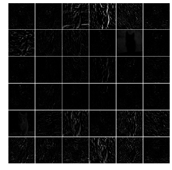
来看看第1个卷积层的输出数据(只显示了前36个)：

 
 

   
   

    
    

   
   
   
   

    
    

     
     feat = net.blobs[
     
     'conv1'].data[
     
     0, :
     
     36]
    
    
   
   

   
   

    
    

   
   
   
   

    
    

     
     vis_square(feat)
    
    
   
   
 
 

同样的道理，想要显示第5个卷积层相应的数据，第5个pooling层的数据，等都是一样的。

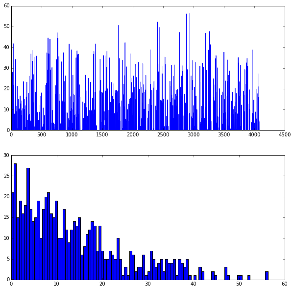
那么全连接层的数据怎么显示呢？

以fc6的输出为例：

 
 

   
   

    
    

   
   
   
   

    
    

     
     feat = net.blobs[
     
     'fc6'].data[
     
     0]
    
    
   
   

   
   

    
    

   
   
   
   

    
    

     
     plt.subplot(
     
     2, 
     
     1, 
     
     1)
    
    
   
   

   
   

    
    

   
   
   
   

    
    

     
     plt.plot(feat.flat)
    
    
   
   

   
   

    
    

   
   
   
   

    
    

     
     plt.subplot(
     
     2, 
     
     1, 
     
     2)
    
    
   
   

   
   

    
    

   
   
   
   

    
    

     
     _ = plt.hist(feat.flat[feat.flat > 
     
     0], bins=
     
     100)
    
    
   
   
 
 

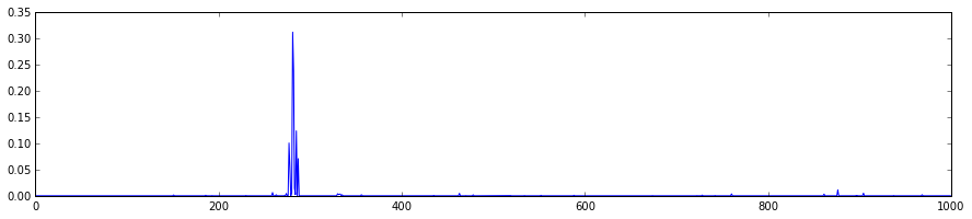
最后希望将所有分类的概率都画出来：

 
 

   
   

    
    

   
   
   
   

    
    

     
     feat = net.blobs[
     
     'prob'].data[
     
     0]
    
    
   
   

   
   

    
    

   
   
   
   

    
    

     
     plt.figure(figsize=(
     
     15, 
     
     3))
    
    
   
   

   
   

    
    

   
   
   
   

    
    

     
     plt.plot(feat.flat)
    
    
   
   
 
 

[<matplotlib.lines.Line2D at 0x7f09587dfb50>]