本篇文章大部分内容翻译自learning pytorch with examples。

1.PyTorch介绍

PyTorch是使用GPU和CPU优化的深度学习张量库，该项目2017年1月由facebook开源，短短两年时间，github上星数已经有25000+，增长速度非常快。

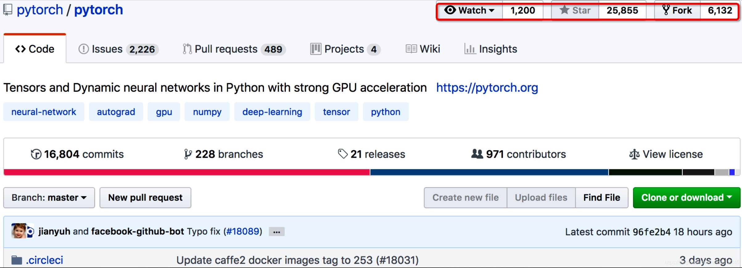
PyTorch的底层和Torch框架一样，但是使用Python重新写了很多内容，不仅更加灵活，支持动态图，而且提供了Python接口。是一个以Python优先的深度学习框架，PyTorch既可以看作加入了GPU支持的numpy，同时也可以看成一个拥有自动求导功能的强大的深度神经网络。除了Facebook外，它已经被Twitter、CMU和Salesforce等机构采用。最近看到大神贾清扬的一段采访，说目前facebook一半以上的应用使用pytorch搭建，fb对此的投入还是很大的。

下面代码来自文献2官方的example，说说深度学习与反向传播及python如何实现。输入batch为64，长度为1000的张量，经过FC + ReLU + FC，损失函数定义为MSE，输出batch为64，长度为10的张量。

2.examples

（1）numpy实现

numpy是python进行数值计算的库，这个库中主要的处理都是由C和C++实现的，因此效率还是很高的。

import numpy as np

# N is batch size; D_in is input dimension;
# H is hidden dimension; D_out is output dimension.
N, D_in, H, D_out = 64, 1000, 100, 10

# Create random input and output data
x = np.random.randn(N, D_in)        #64*1000
y = np.random.randn(N, D_out)       #64*10

# Randomly initialize weights
w1 = np.random.randn(D_in, H)       #1000*100
w2 = np.random.randn(H, D_out)      #100*10

learning_rate = 1e-6
for t in range(500):
    # Forward pass: compute predicted y
    h = x.dot(w1)       #same to np.dot(x,w1), h:64*100
    h_relu = np.maximum(h, 0)       #64*100
    y_pred = h_relu.dot(w2)         #64*10

    # Compute and print loss
    loss = np.square(y_pred - y).sum()
    print(t, loss)

    # Backprop to compute gradients of w1 and w2 with respect to loss
    grad_y_pred = 2.0 * (y_pred - y)
    grad_w2 = h_relu.T.dot(grad_y_pred)     #h_relu.T is the transpose of h_relu，也就是转置,h_relu.T:100*64
    grad_h_relu = grad_y_pred.dot(w2.T)
    grad_h = grad_h_relu.copy()
    grad_h[h < 0] = 0
    grad_w1 = x.T.dot(grad_h)

    # Update weights
    w1 -= learning_rate * grad_w1
    w2 -= learning_rate * grad_w2

代码保存为test2.py，运行结果如下，收敛还是很快的。

（2）PyTorch实现

这里需安装pytorch，参考官方教程安装就好，我的环境使用anaconda来安装的，需要说明的是，pytorch支持cpu和gpu，通过torch.device可以很方便的切换。

Numpy是一个很好用的库，但它不能利用GPU来加速其数值计算。对于深度神经网络来说，GPU通常提供50倍或更高的加速。而使用PyTorch可以利用GPU来加速，Tensor(张量）是PyTorch中最基本的概念，其实就是一个n维数组，Pytorch提供了与Tensor相关的很多操作，并且都可以在GPU上实现。

与numpy不同，PyTorch Tensors可以利用GPU加速其数值计算。要在GPU上运行PyTorch Tensor，只需将其转换为新的数据类型即可。

下面的代码将实现与上面NumPy相同的功能

import torch

dtype = torch.float
device = torch.device("cpu")
# device = torch.device("cuda:0") # Uncomment this to run on GPU

# N is batch size; D_in is input dimension;
# H is hidden dimension; D_out is output dimension.
N, D_in, H, D_out = 64, 1000, 100, 10

# Create random Tensors to hold input and outputs.
# Setting requires_grad=False indicates that we do not need to compute gradients
# with respect to these Tensors during the backward pass.
x = torch.randn(N, D_in, device=device, dtype=dtype)
y = torch.randn(N, D_out, device=device, dtype=dtype)

# Create random Tensors for weights.
# Setting requires_grad=True indicates that we want to compute gradients with
# respect to these Tensors during the backward pass.
w1 = torch.randn(D_in, H, device=device, dtype=dtype, requires_grad=True)
w2 = torch.randn(H, D_out, device=device, dtype=dtype, requires_grad=True)

learning_rate = 1e-6
for t in range(500):
    # Forward pass: compute predicted y using operations on Tensors; these
    # are exactly the same operations we used to compute the forward pass using
    # Tensors, but we do not need to keep references to intermediate values since
    # we are not implementing the backward pass by hand.
    y_pred = x.mm(w1).clamp(min=0).mm(w2)

    # Compute and print loss using operations on Tensors.
    # Now loss is a Tensor of shape (1,)
    # loss.item() gets the a scalar value held in the loss.
    loss = (y_pred - y).pow(2).sum()
    print(t, loss.item())

    # Use autograd to compute the backward pass. This call will compute the
    # gradient of loss with respect to all Tensors with requires_grad=True.
    # After this call w1.grad and w2.grad will be Tensors holding the gradient
    # of the loss with respect to w1 and w2 respectively.
    loss.backward()

    # Manually update weights using gradient descent. Wrap in torch.no_grad()
    # because weights have requires_grad=True, but we don't need to track this
    # in autograd.
    # An alternative way is to operate on weight.data and weight.grad.data.
    # Recall that tensor.data gives a tensor that shares the storage with
    # tensor, but doesn't track history.
    # You can also use torch.optim.SGD to achieve this.
    with torch.no_grad():
        w1 -= learning_rate * w1.grad
        w2 -= learning_rate * w2.grad

        # Manually zero the gradients after updating weights
        w1.grad.zero_()
        w2.grad.zero_()

（3）PyTorch AutoGrad实现

在前面的介绍中，我们需要手动实现前向网络forward和反向网络backward，对两层网络来说，很好实现，但对于分类、检测、分割等比较复杂的深度学习网络来说，就显得不够优雅了。

在PyTorch中，我们可以使用AutoGrad包，利用automatic differentation方法来自动计算backward，使用AutoGrad包时，前向网络定义了一套计算图，使用计算图来执行，计算图中的每个节点都定义为Tensors，通过这个计算图反向传播可以比较容易计算得到梯度值。

也就是说，如果x是一个张量，并且x.requires_grad=True，那么x.grad是对应x的梯度值的张量，下面来看利用AutoGrad库实现的两层网络。

import torch

dtype = torch.float
device = torch.device("cpu")
# device = torch.device("cuda:0") # Uncomment this to run on GPU

# N is batch size; D_in is input dimension;
# H is hidden dimension; D_out is output dimension.
N, D_in, H, D_out = 64, 1000, 100, 10

# Create random Tensors to hold input and outputs.
# Setting requires_grad=False indicates that we do not need to compute gradients
# with respect to these Tensors during the backward pass.
x = torch.randn(N, D_in, device=device, dtype=dtype)
y = torch.randn(N, D_out, device=device, dtype=dtype)

# Create random Tensors for weights.
# Setting requires_grad=True indicates that we want to compute gradients with
# respect to these Tensors during the backward pass.
w1 = torch.randn(D_in, H, device=device, dtype=dtype, requires_grad=True)
w2 = torch.randn(H, D_out, device=device, dtype=dtype, requires_grad=True)

learning_rate = 1e-6
for t in range(500):
    # Forward pass: compute predicted y using operations on Tensors; these
    # are exactly the same operations we used to compute the forward pass using
    # Tensors, but we do not need to keep references to intermediate values since
    # we are not implementing the backward pass by hand.
    y_pred = x.mm(w1).clamp(min=0).mm(w2)

    # Compute and print loss using operations on Tensors.
    # Now loss is a Tensor of shape (1,)
    # loss.item() gets the a scalar value held in the loss.
    loss = (y_pred - y).pow(2).sum()
    print(t, loss.item())

    # Use autograd to compute the backward pass. This call will compute the
    # gradient of loss with respect to all Tensors with requires_grad=True.
    # After this call w1.grad and w2.grad will be Tensors holding the gradient
    # of the loss with respect to w1 and w2 respectively.
    loss.backward()

    # Manually update weights using gradient descent. Wrap in torch.no_grad()
    # because weights have requires_grad=True, but we don't need to track this
    # in autograd.
    # An alternative way is to operate on weight.data and weight.grad.data.
    # Recall that tensor.data gives a tensor that shares the storage with
    # tensor, but doesn't track history.
    # You can also use torch.optim.SGD to achieve this.
    with torch.no_grad():
        w1 -= learning_rate * w1.grad
        w2 -= learning_rate * w2.grad

        # Manually zero the gradients after updating weights
        w1.grad.zero_()
        w2.grad.zero_()

非常的简单就实现了两层网络。
至繁归于至简！

参考：
[1] https://github.com/pytorch/pytorch
[2] https://pytorch.org/tutorials/beginner/pytorch_with_examples.html
[3] https://baijiahao.baidu.com/s?id=1590200756011465121&wfr=spider&for=pc