社区检测

进入研一开始接触到图神经网络，其中自然逃不过社区检测这一经典问题。社区检测(community detection)又被称为是社区发现，它是用来揭示网络聚集行为的一种技术。社区检测实际就是一种网络聚类的方法，通俗来讲就是将具有相同特性和不同特性的节点进行结构划分。
网络社区划分的优劣往往通过模块度来进行衡量。一个网络不通情况下的社区划分对应不同的模块度。模块度越大，对应的社区划分也就越合理;如果模块度越小，则对应的网络社区划分也就越模糊。本项目采用模块度作为优化的目标，其计算函数会在下面进行一定的解释。
下面基于Pytorch Geometric对本文的社区检测进行复现。如果有朋友想要学习使用networkx作为代替对本论文进行复现，可以参考我师兄的文章，里面的讲解非常清晰：PyTorch图神经网络实践（七）社区检测

论文介绍——端到端的学习与优化

这篇文章《End to end learning and optimization on graphs》2019年发表在人工智能和机器学习领域的国际顶级会议 NeurIPS上。在之前的传统方法中，往往是先对对图的学习问题进行解决，再进行优化。在实际应用中，图的学习和优化问题常常是结合在一起，比如图或相关属性往往只是部分观察到，引入了一些学习问题，如链接预测，必须在优化之前解决。文章作者提出了一种端到端的方法，将学习问题和优化问题结合到了一起，将优化问题作为学习任务的一层，运用下游的优化误差反过来传递到学习的任务上，这允许模型特别关注下游任务，它的预测将用于该任务。
实验结果表明，作者的ClusterNet系统优于纯端到端方法（直接预测最优解决方案）和完全分离学习和优化的标准方法。
作者源码见GitHub：https://github.com/bwilder0/clusternet

技术方法ClusterNet

作者以链路预测和社区检测分别作为学习任务和优化任务。
引用我师兄的解释，具体上，文章假定在进行社区检测之前，网络结构不是完全已知的，只有部分（40%）网络结构是能够观察到的，所以要先用链路预测来找出出网络中那些没有被观察到的连边，然后再在这种“复原”后的网络上进行社区检测，利用模块度指标来评估社区检测的效果。同时，文章还设立了对照实验，即在原始网络（不隐藏任何连边）上执行社区检测任务，通过观察两组实验的结果来分析他们提出的模型的有效性。这种学习+优化的任务复现可以看后一篇博客《利用PyG实现端到端的链路预测+社区检测（组合优化》 。
在文中，作者提出了一种端到端的模型ClusterNet，先让数据经过两层GCN进行嵌入，再将卷积网络的输出放入K means聚类函数中进行迭代聚类，最后运用输出的分配矩阵和模块度进行损失计算（即优化目标），反向传递并进行参数优化。
在本人看来，核心在于在其中将优化任务作为学习任务中的一层进行误差的反向传播。
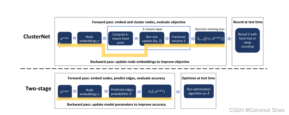
模型结构如下图所示：
上图：ClusterNet，下图：典型的学习+优化两阶段方法。
特别注意的是，在K means聚类中我们可以得到软分配矩阵， 在训练过程中我们在softmax过程中会进行软分配，即用概率来描述节点分配到不同簇的概率，这样对参数的优化会更为准确；而在测试过程中，我们会加大softmax的硬度（hard）系数，甚至每一百轮使用100作为硬度系数（代码中也叫cluster_temp）来对r进行乘积再进行softmax操作，使其变为非0即1的硬划分。 这样对分配结果有更好的展示，也可以计算实际的预测损失。
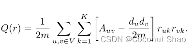
在ClusterNet中，作者使用模块度作为优化的目标，具体公式如下：

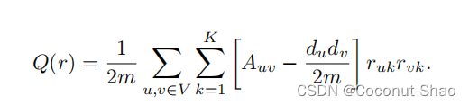
其中r为软分配矩阵，d为节点的度，A为邻接矩阵。具体的计算过程会在下面代码讲解的地方讲到。

作者在多个不同数据集上进行了测试。为了方便对比，作者设计了一种没有聚类的端到端方法GCN-e2e，这种方法可以视为将所有的节点视为一个社区，这样便没有外部节点，也算是一种最优。对比可以看出，聚类的存在可以将精度大幅提升：

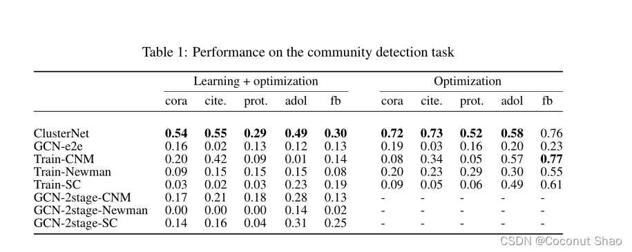
这也进一步证明了聚类层在社区检测任务中的不可或缺。
下面将使用PyG对Cora数据集进行纯优化的复现。非常有意思的是，下面将会讲到Cora中的节点一共具有7个类别，但是在聚类过程中将其归为五簇（聚类系数K设为5）的效果最好。个人猜测是因为有两类节点的数目相对较少，如果单独划出的话会影响各个簇的平衡以及整体的划分精度，每个类的匹配程度会相对减弱，所以舍小保大。

基于Cora数据集复现ClusterNet优化部分代码

我们选择在Cora数据集上进行论文优化部分的代码复现。Cora数据集是图优化问题的一个经典的单图数据集，来源于论文Revisiting Semi-Supervised Learning with Graph Embeddings，包含2708篇科学出版物， 10556条边，每个节点有其独自的类别，总共7种类别。数据集中的每个出版物都由一个 0/1 值的词向量描述，表示字典中相应词的缺失/存在。 该词典由 1433 个独特的词组成。意思就是说每一个出版物都由1433个特征构成，每个特征仅由0/1表示。PyG中Cora数据集的具体的参数如下图：

在实现数据集引入和处理方面，本人主要使用了PyTorch Geometric这个库，这是我的大牛师兄推荐的一个比较简单的处理图问题的函数库，它的函数兼容性好并且操作相比于networkx较为简单（个人感觉哈），内置了大量数据集的自下载及其处理方式。具体介绍可以见官网：https://pytorch-geometric.readthedocs.io/en/latest/

导入需要的包

from torch_geometric.datasets import Planetoid
import torch
import torch.nn.functional as F
from torch_geometric.nn import GCNConv
import numpy as np
import scipy.sparse as sp
from models import cluster, GCNClusterNet, GCN

这里我们直接使用PyG内自带的GCN卷积核，这个类的输入为PyG格式的edge_index，而不需要提前转换成adj的邻接矩阵格式，可以说是数据集拿过来不用处理就可以做卷积，非常的便捷。

导入Cora数据集

这里利用PyG的格式直接导入Cora数据集：

dataset = Planetoid(root='../tmp/Cora', name='Cora')
device = torch.device('cuda' if torch.cuda.is_available() else 'cpu')
data = dataset[0].to(device)

运行完之后可以看到，在data中的参数分别为：edge_index=[2, 10556], test_mask=[2708],
train_mask=[2708], val_mask=[2708], x=[2708, 1433], y=[2708]。具体的代表意义上述PyG官网有详细的例子，讲解的非常清晰。可以看到，这里对边的存储格式并不是以邻接矩阵adj的2708x2708的形式，而是直接用相连边的起点和终点构成的2x10556。

数据处理和模型搭建

本人运用PyG找到一种比作者更为便捷和节省的方法，可以避免许多冗杂的数据处理方式，并且测试过后优化的精度不变。两种方法都基于PyG，主要区别是GCNClusterNet中embeds的获得方式不同。第二种方法引入了一些数据处理方式来将PyG的图格式转换为了特征矩阵和邻接矩阵再接入传统的GCN，第一种方法直接使用PyG格式的GCN。均放在这里进行讲解供大家选择。
两种方法返回参数的均为 ：
embeds——节点embedding，即未经历cluster进行K means的GCN输出，维度为节点数量xGCN的输出层，即2708x50；
mu——cluster means，维度为聚类系数Kx输出层，即5x50;
r——软分配矩阵，维度为节点数量x聚类系数K，即2708x5；
dist——节点相似性，即每个点到每个簇中心的距离，维度为节点数量x聚类系数K，即2708x5。

GCNClusterNet的初始化参数分别为：
nfeat——图的节点特征维度,；
nhid=50——双层GCN隐藏层维度,；
nout=50——双层GCN输出层维度；
dropout=0.2——双层GCNdropout参数；
K=5——聚类的cluster数量；
cluster_temp=50——softmax后的突出程度即硬度系数，官方解释为：how hard to make the softmax for the cluster assignments。
具体的输出层维度隐藏层维度等参数在模型训练代码的第一行指定。

方法一（PyG简洁版）

只需要用PyG构建一个两层的GCN，然后在GCNClusterNet中调用数据集即data即可得到embeds。

class GCN_NET(torch.nn.Module):
    def __init__(self, nhid, nout, dropout):
        super().__init__()
        self.conv1 = GCNConv(dataset.num_node_features, nhid)
        self.conv2 = GCNConv(nhid,nout)
        self.dropout = dropout
    def forward(self, data):
        x, edge_index = data.x, data.edge_index
        x = self.conv1(x, edge_index)
        x = F.relu(x)
        x = F.dropout(x,self.dropout , training=self.training)
        x = self.conv2(x, edge_index)
        return x


class GCNClusterNet(torch.nn.Module):
	    '''
    The ClusterNet architecture. The first step is a 2-layer GCN to generate embeddings.
    The output is the cluster means mu and soft assignments r, along with the
    embeddings and the the node similarities (just output for debugging purposes).

    The forward pass inputs are x, a feature matrix for the nodes, and adj, a sparse
    adjacency matrix. The optional parameter num_iter determines how many steps to
    run the k-means updates for.
    '''
    def __init__(self, nfeat, nhid, nout, dropout, K, cluster_temp):
        super(GCNClusterNet, self).__init__()
        self.GCN_NET = GCN_NET(nhid, nout, dropout)
        self.distmult = torch.nn.Parameter(torch.rand(nout))
        self.sigmoid = torch.nn.Sigmoid()
        self.K = K
        self.cluster_temp = cluster_temp
        self.init = torch.rand(self.K, nout)

    def forward(self,x,adj, num_iter=1):
    	#这里的x，adj没有用，为了方便对比本人把它们作为参数加了进来
        embeds = self.GCN_NET(data)
        mu_init, _, _ = cluster(embeds, self.K, 1, num_iter, cluster_temp=self.cluster_temp, init=self.init)
        mu, r, dist = cluster(embeds, self.K, 1, 1, cluster_temp=self.cluster_temp, init=mu_init.detach().clone())
        return mu, r, embeds, dist

方法二（PyG复杂版）

先对图取特征和边数据，生成特征矩阵和邻接矩阵，再进行归一化操作并转化为tensor类型，送入GCN中得到embeds。

def normalize(mx):
	"""Row-normalize sparse matrix"""
    rowsum = np.array(mx.sum(1))  # 矩阵行求和
    r_inv = np.power(rowsum, -1).flatten()  # 每行和的-1次方
    r_inv[np.isinf(r_inv)] = 0.  # 如果是inf，转换为0
    r_mat_inv = sp.diags(r_inv)  # 转换为对角阵
    mx = r_mat_inv.dot(mx)  # D-1*A,乘上特征，按行归一化
    return mx


def sparse_mx_to_torch_sparse_tensor(sparse_mx):
	"""Convert a scipy sparse matrix to a torch sparse tensor."""
    sparse_mx = sparse_mx.tocoo().astype(np.float32)
    indices = torch.from_numpy(
        np.vstack((sparse_mx.row, sparse_mx.col)).astype(np.int64))
    values = torch.from_numpy(sparse_mx.data)
    shape = torch.Size(sparse_mx.shape)
    return torch.sparse.FloatTensor(indices, values, shape)


features = sp.csr_matrix(data.x, dtype=np.float32)  # 取特征
adj = sp.coo_matrix((np.ones(data.edge_index.shape[1]), (data.edge_index[0, :], 			data.edge_index[1, :])),
                    shape=(data.y.shape[0], data.y.shape[0]), dtype=np.float32)
adj = adj + adj.T.multiply(adj.T > adj) - adj.multiply(adj.T > adj)
features = normalize(features)  # 特征归一化
adj = normalize(adj + sp.eye(adj.shape[0]))  # A+I归一化
features = torch.FloatTensor(np.array(features.todense()))# 将numpy的数据转换成torch格式
adj = sparse_mx_to_torch_sparse_tensor(adj)
adj = adj.coalesce()
bin_adj_all = (adj.to_dense() > 0).float()
class GCNClusterNet(torch.nn.Module):
    def __init__(self, nfeat, nhid, nout, dropout, K, cluster_temp):
        super(GCNClusterNet, self).__init__()
        self.GCN = GCN(nfeat, nhid, nout, dropout)
        self.distmult = torch.nn.Parameter(torch.rand(nout))
        self.sigmoid = torch.nn.Sigmoid()
        self.K = K
        self.cluster_temp = cluster_temp
        self.init = torch.rand(self.K, nout)

    def forward(self, x,adj, num_iter=1):
        embeds = self.GCN(x, adj)
        mu_init, _, _ = cluster(embeds, self.K, 1, num_iter, cluster_temp=self.cluster_temp, init=self.init)
        mu, r, dist = cluster(embeds, self.K, 1, 1, cluster_temp=self.cluster_temp, init=mu_init.detach().clone())
        return mu, r, embeds, dist

模块度矩阵函数和损失函数（优化目标）

在模块度矩阵函数中，先对邻接矩阵进行对角线清0，再求和生成度矩阵，最后将二者带入论文的公式中生产模块度矩阵（分类好坏的评价标准）。
在损失函数中，利用软分配矩阵r，归一化后的邻接矩阵bin_adj模块度矩阵mod带入论文中的公式求得模块度损失，即我们优化的目标。

def make_modularity_matrix(adj):
    adj = adj * (torch.ones(adj.shape[0], adj.shape[0]) - torch.eye(adj.shape[0]))
    degrees = adj.sum(axis=0).unsqueeze(1)
    mod = adj - degrees @ degrees.t() / adj.sum()
    return mod


def loss_modularity(r, bin_adj, mod):
    bin_adj_nodiag = bin_adj * (torch.ones(bin_adj.shape[0], bin_adj.shape[0]) - torch.eye(bin_adj.shape[0]))
    return (1. / bin_adj_nodiag.sum()) * (r.t() @ mod @ r).trace()

模型训练

首先我们利用模块度矩阵函数得到我们的测试对象——模块度，命名为test_object，并且对r，归一化后的adj，test_object计算loss损失，取负数逆向求导，对参数进行优化。
当训练到500轮时，num_iter更改为5，增加cluster的迭代次数（K means更新的步骤数）。
每100轮迭代，观察是否改善最佳的培训损失。其中我们对测试的softmax直接使用cluster_temp=100来突出其分配程度（相当于软分配转换为了硬分配）。

model_cluster = GCNClusterNet(nfeat=1433, nhid=50, nout=50, dropout=0.2, K=5, cluster_temp=50)
optimizer = torch.optim.Adam(model_cluster.parameters(), lr=0.01, weight_decay=5e-4)
test_object = make_modularity_matrix(bin_adj_all)
model_cluster.train()
num_cluster_iter = 1
losses = []
for epoch in range(1001):
    mu, r, embeds, dist = model_cluster(features, adj, num_cluster_iter)
    loss = loss_modularity(r, bin_adj_all, test_object)
    loss = -loss
    optimizer.zero_grad()
    loss.backward()
    if epoch == 500:
        num_cluster_iter = 5
    if epoch % 100 == 0:
        r = torch.softmax(100 * r, dim=1)
    loss_test = loss_modularity(r, bin_adj_all, test_object)
    if epoch == 0:
        best_train_val = 100
    if loss.item() < best_train_val:
        best_train_val = loss.item()
        curr_test_loss = loss_test.item()
        # convert distances into a feasible (fractional x)#将距离转换为可行的（分数x）
        x_best = torch.softmax(dist * 100, 0).sum(dim=1)
        x_best = 2 * (torch.sigmoid(4 * x_best) - 0.5)
        if x_best.sum() > 5:
            x_best = 5 * x_best / x_best.sum()
    losses.append(loss.item())
    optimizer.step()
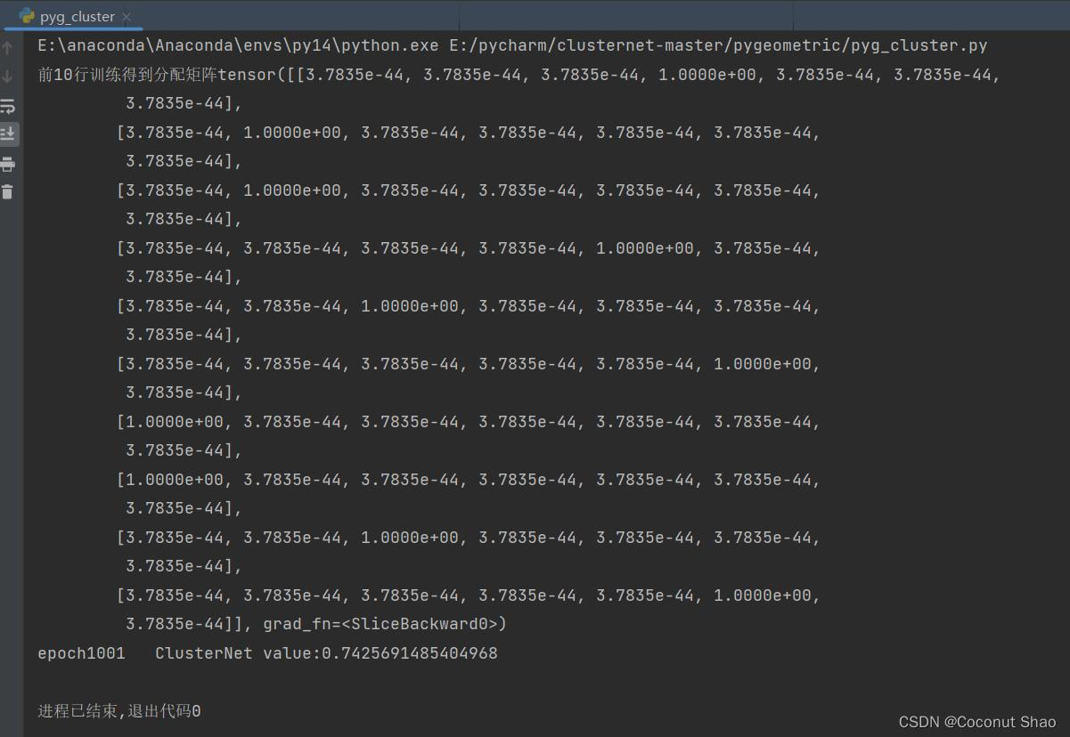
print(f'epoch{epoch + 1}   ClusterNet value:{curr_test_loss}')

最后输出优化的精度为：0.716，与作者论文中的精度几乎一致。

基于Cora数据集复现ClusterNet链路预测+优化部分代码

上面，我们虽然将优化任务作为学习任务中的一层进行误差的反向传播，但实际情况中，网络结构不是完全已知的，只有部分（假设40%）网络结构是能够观察到的，所以要先用链路预测来找出出网络中那些没有被观察到的连边，然后再在这种“复原”后的网络上进行社区检测，利用模块度指标来评估社区检测的效果。

我们仍然使用PyG来对论文进行复现，在模型搭建上，我们选择上述的方法一，我们同样通过PyG的内置函数来对边进行划分。在对边进行40%提取时采用了PyG的内置函数：train_test_split_edges，有效减少了40%边构建邻接矩阵的复杂度。
与上面纯优化不同的是，我们输入模型进行训练的是数量为实际边数40%的链接，从而得到的软分配矩阵为用40%链接训练得出的r。在训练过程中也是采用这40%的边构建的归一化邻接矩阵adj_train来计算模块度train_object，并对模块度train_object，训练得出的软分配矩阵r和adj_train来进行损失计算和误差的反向传播——这就是链路预测（学习任务）之后用模块度目标（优化目标）来对链路预测的参数进行更新。
同时，我们在测试时，会将用train_object训练出来的分配矩阵r进行硬化（即用非常大的硬度系数使其变为硬分配矩阵，如前面概念所讲），与到test_object（所有边计算出的的模块度）计算损失，来验证分配结的社区结果在全图上的结果和精度。
其余函数和代码结构与纯优化相同，不作具体解释。所有代码如下：

from torch_geometric.datasets import Planetoid
import torch
import torch.nn.functional as F
from torch_geometric.nn import GCNConv
import numpy as np
import scipy.sparse as sp
from models import cluster, GCNClusterNet, GCN
from torch_geometric.utils import train_test_split_edges



def normalize(mx):
    rowsum = np.array(mx.sum(1))  # 矩阵行求和
    r_inv = np.power(rowsum, -1).flatten()  # 每行和的-1次方
    r_inv[np.isinf(r_inv)] = 0.  # 如果是inf，转换为0
    r_mat_inv = sp.diags(r_inv)  # 转换为对角阵
    mx = r_mat_inv.dot(mx)  # D-1*A,乘上特征，按行归一化
    return mx


def sparse_mx_to_torch_sparse_tensor(sparse_mx):
    sparse_mx = sparse_mx.tocoo().astype(np.float32)
    indices = torch.from_numpy(
        np.vstack((sparse_mx.row, sparse_mx.col)).astype(np.int64))
    values = torch.from_numpy(sparse_mx.data)
    shape = torch.Size(sparse_mx.shape)
    return torch.sparse.FloatTensor(indices, values, shape)


class GCN_NET(torch.nn.Module):
    def __init__(self,nfeat,nhid, nout, dropout):
        super().__init__()
        self.conv1 = GCNConv(nfeat, nhid)
        self.conv2 = GCNConv(nhid,nout)
        self.dropout = dropout
    def forward(self, data,pure_opt):
        if pure_opt:
            x, edge_index = data.x, data.edge_index
        else:
            x , edge_index = data.x, data.train_pos_edge_index

        x = self.conv1(x, edge_index)
        x = F.relu(x)
        x = F.dropout(x,self.dropout , training=self.training)
        x = self.conv2(x, edge_index)
        return x


class GCNClusterNet(torch.nn.Module):
    def __init__(self, nfeat, nhid, nout, dropout, K, cluster_temp):#nfeat=1433, nhid=50, nout=50, dropout=0.2, K=5, cluster_temp=50
        super(GCNClusterNet, self).__init__()
        self.GCN_NET = GCN_NET(nfeat,nhid, nout, dropout)
        self.distmult = torch.nn.Parameter(torch.rand(nout))
        self.sigmoid = torch.nn.Sigmoid()
        self.K = K
        self.cluster_temp = cluster_temp
        self.init = torch.rand(self.K, nout)

    def forward(self, data, num_iter=1, pure_opt=False):
        embeds = self.GCN_NET(data,pure_opt)
        mu_init, _, _ = cluster(embeds, self.K, 1, num_iter, cluster_temp=self.cluster_temp, init=self.init)
        mu, r, dist = cluster(embeds, self.K, 1, 1, cluster_temp=self.cluster_temp, init=mu_init.detach().clone())
        return mu, r, embeds, dist


def make_modularity_matrix(adj):
    adj = adj * (torch.ones(adj.shape[0], adj.shape[0]) - torch.eye(adj.shape[0]))
    degrees = adj.sum(axis=0).unsqueeze(1)
    # degrees = torch.unsqueeze(degrees,1)
    mod = adj - degrees @ degrees.t() / adj.sum()
    return mod


def loss_modularity(r, bin_adj, mod):
    bin_adj_nodiag = bin_adj * (torch.ones(bin_adj.shape[0], bin_adj.shape[0]) - torch.eye(bin_adj.shape[0]))
    return (1. / bin_adj_nodiag.sum()) * (r.t() @ mod @ r).trace()


pure_opt = False
K = 7
dataset = Planetoid(root='../tmp/Cora', name='Cora')
device = torch.device('cuda' if torch.cuda.is_available() else 'cpu')
data = dataset[0].to(device)

features = sp.csr_matrix(data.x, dtype=np.float32)  # 取特征
adj = sp.coo_matrix((np.ones(data.edge_index.shape[1]), (data.edge_index[0, :], data.edge_index[1, :])),
                    shape=(data.y.shape[0], data.y.shape[0]), dtype=np.float32)
adj = adj + adj.T.multiply(adj.T > adj) - adj.multiply(adj.T > adj)
features = normalize(features)  # 特征归一化
adj = normalize(adj + sp.eye(adj.shape[0]))  # A+I归一化
# 将numpy的数据转换成torch格式
features = torch.FloatTensor(np.array(features.todense()))
# labels_np = data.y.numpy
# labels = torch.LongTensor(labels_np) #[1]
adj = sparse_mx_to_torch_sparse_tensor(adj)
adj = adj.coalesce()
bin_adj_all = (adj.to_dense() > 0).float()
test_object = make_modularity_matrix(bin_adj_all)
num_cluster_iter = 1
losses = []
val_ratio=0.3
test_ratio=0.3
if not pure_opt:
    data = train_test_split_edges(data, val_ratio=val_ratio,test_ratio=test_ratio)
    model_cluster = GCNClusterNet(nfeat=data.x.size(1), nhid=50, nout=50, dropout=0.2, K=K, cluster_temp=50)

    adj_train = sp.coo_matrix((np.ones(data.train_pos_edge_index.shape[1]), (data.train_pos_edge_index[0, :], data.train_pos_edge_index[1, :])),
                        shape=(data.y.shape[0], data.y.shape[0]), dtype=np.float32)
    adj_train = adj_train + adj_train.T.multiply(adj_train.T > adj_train) - adj_train.multiply(adj_train.T > adj_train)
    adj_train = normalize(adj_train + sp.eye(adj_train.shape[0]))
    adj_train = sparse_mx_to_torch_sparse_tensor(adj_train)
    adj_train = adj_train.coalesce()
    bin_adj_train = (adj_train.to_dense() > 0).float()
    train_object = make_modularity_matrix(bin_adj_train)
else:
    model_cluster = GCNClusterNet(nfeat=data.x.size(1), nhid=50, nout=50, dropout=0.2, K=K, cluster_temp=50)
# model_cluster.train()
optimizer = torch.optim.Adam(model_cluster.parameters(), lr=0.01, weight_decay=5e-4)

for epoch in range(1001):
    mu, r, embeds, dist = model_cluster(data, num_cluster_iter, pure_opt=False)
    if not pure_opt:
        loss = loss_modularity(r, bin_adj_train, train_object)
    else:
        loss = loss_modularity(r, bin_adj_all, test_object)
    loss = -loss
    optimizer.zero_grad()
    loss.backward()
    if epoch == 500:
        num_cluster_iter = 5
    if epoch % 100 == 0:
        r = torch.softmax(100 * r, dim=1)
        if epoch ==1000:
            print(f"前10行训练得到分配矩阵{r[0:10,0:K]}")
    loss_test = loss_modularity(r, bin_adj_all, test_object)
    if epoch == 0:
        best_train_val = 100
    if loss.item() < best_train_val:
        best_train_val = loss.item()
        curr_test_loss = loss_test.item()
        # convert distances into a feasible (fractional x)#将距离转换为可行的（分数x）
        x_best = torch.softmax(dist * 100, 0).sum(dim=1)
        x_best = 2 * (torch.sigmoid(4 * x_best) - 0.5)
        if x_best.sum() > 5:
            x_best = 5 * x_best / x_best.sum()
    losses.append(loss.item())
    optimizer.step()

print(f'epoch{epoch + 1}   ClusterNet value:{curr_test_loss}')
if not pure_opt:
    print(f"链路预测+优化，已知{1.0-test_ratio-val_ratio}的边")

设置K=7时和K=5时的分配结果相似。当K=7时，输出结果如下图所示：

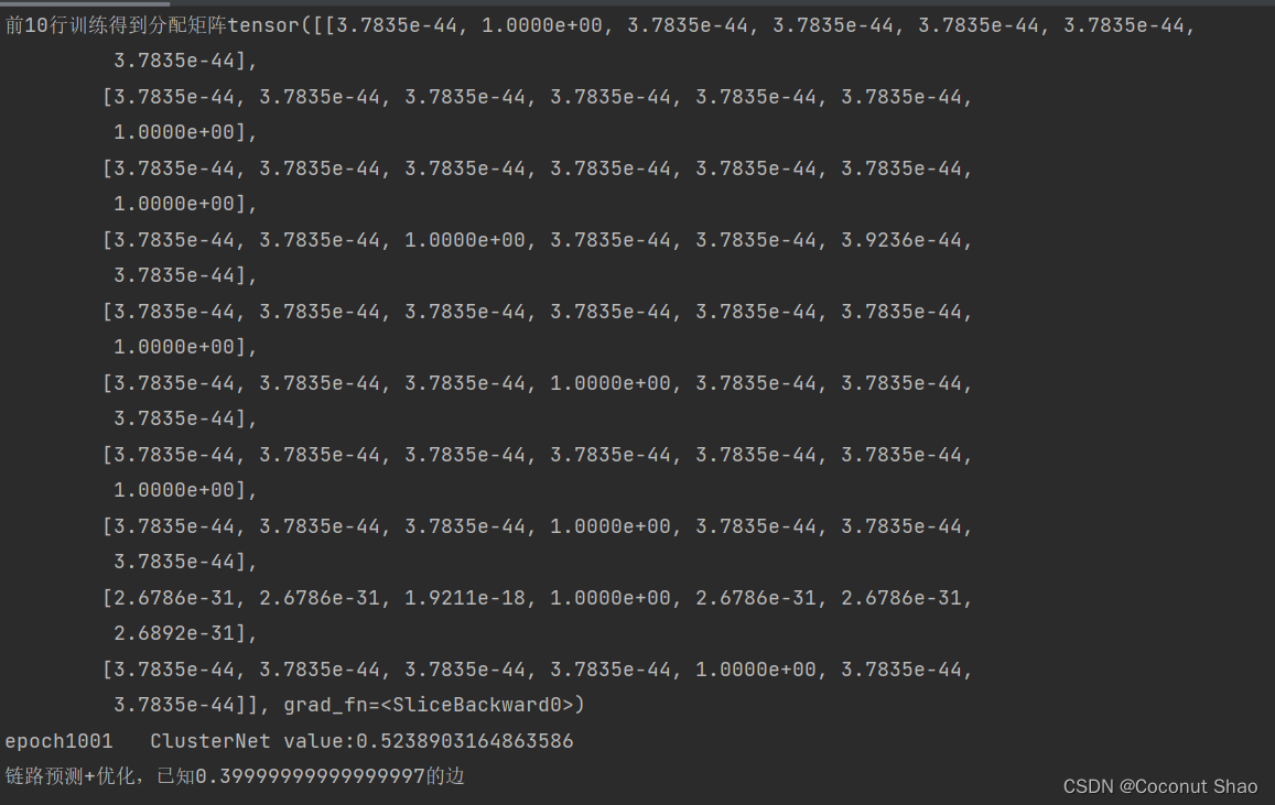
对比论文中的0.54，我们得到的0.52在合理误差范围内，可以认为结果一致。

补充

作者在原代码中使用的为40%的节点的特征和40%的边，而我们这里在GCN输入训练的为所有的节点的特征和40%的边，得到的结果差距不大。这也表明了链接和标签/特征的关系不大。推测该数据集标签与链接反映的信息不一样，有可能不同类别之间存在很多链接，而同类别中的链接占比不高。
为了测试该猜想，我们将完整的标签作为分配矩阵与所有边得出的模块度test_object进行优化计算（纯优化过程），得到社区分配的分数为0.64，甚至小于训练得出的分配数值。这有可能验证上述的猜想。


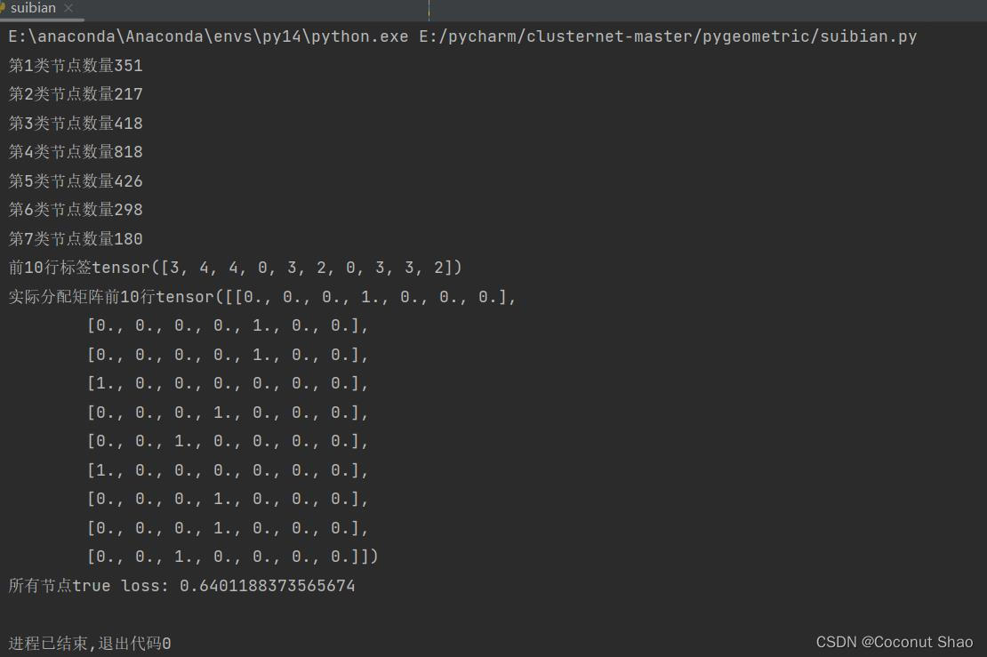
上图为训练得到的分数，下图为真实标签作为社区分配得到的分数。